Amp simulation oversampling

In tandem with our last article on Guitar amp simulation, this article gives a step by step view of the sampling and rate conversion processes, with a look at the frequency spectrum.

From guitar to digital

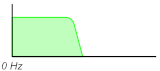
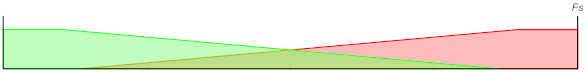
The first two charts embody the initial sampling of the analog signal. It’s done in one step, from your analog-to-digital converter, but it’s a two-part process. First, a lowpass filter clears everything from half the sample rate up—something we must do to avoid higher frequencies aliasing into our audio band when sampled.

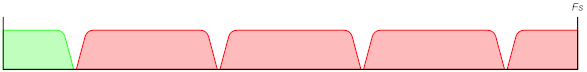
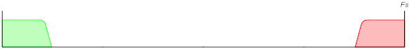
Then the signal is digitized. This creates repeating images of the positive and negative frequencies that extend upward without end. After this, we’ll look only at frequencies between 0 Hz and the sampling frequency, but it’s important to understand that these images are there, nonetheless.

If we don’t need more frequency headroom, we can do our signal processing on the samples we have. In fact, we want to do as much as we can at the lower sample rate. In the case of a guitar amp, we would process any tone controls that come before the “tube”, and other things like DC blocking and noise gating. And we can do our (non-saturating) gain stage here (assuming floating point).

Higher rate processing

After initial processing and gain, it’s time for saturation. For this non-linear process, we need frequency headroom. The first step is to increase the rate by inserting zero-magnitude samples. Though I suggested starting with 8x upsampling in the guitar amp article, this exercise shows 4x, in order to better accommodate page constraints. We place three zero-samples between each existing sample to bring it up 4x. This only raises the sample rate—we have four samples in the same period that we used to have one. Since the spectrum is not altered, the aliases are still there.

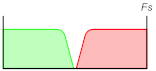
Part two of the sample rate conversion process is to use a lowpass filter to clear everything above our original audio band. (In reality, we optimize the zero insertion and filtering into a single process, to take advantage of multiplies by zero that we can skip. Note we usually use a linear-phase FIR for this step, in order to preserve the wave shape for the saturator.) Now we see our headroom.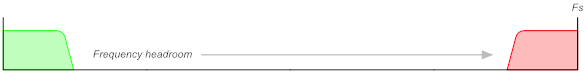

After our saturation stage, we’ve created new harmonics. As long as they are at a sufficiently low level by the time they reach the sample rate minus our final audio bandwidth, the aliased version won’t pollute our audio band.

Back to normal

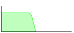
Done with our more expensive high-rate signal processing, we can drop back to our original sample rate for the rest. The first step is to run our lowpass filter again, to clear everything above our audio band.

Part two is the downsampling process—we simply keep one sample, discard three, and repeat. Why did we bother calculating them? Because we needed them ahead of the lowpass filter. But, here also, we can optimize these two down-conversion steps into one, and save needless calculation.

Final processing

From here, we handle other linear processes—any filtering and tone controls the follow the tube stage, effects such spring reverb, and finally the speaker cabinet simulation. In the end, we send it to our digital-to-analog converter, which itself has a lowpass filter to remove the aliased copies.

And enjoy listening.