Further thoughts on wave table oscillators

I see regular questions about wave table oscillators in various forums. While the process is straight forward, I sympathize that it’s not so simple to figure out what’s important if you really want to understand how it works. For instance, the choice of table size and interpolation—how do these affect the oscillator quality? I’ll give an overview here, which I hope helps in thinking about wave table oscillators.

Generating a signal

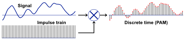
With a goal to generate a tone, we have an idea that instead of computing a tone for an arbitrary amount of time, we can save a lot of setup time and memory by computing just one cycle of the tone at initialization time, storing in a table, and playing it back repeatedly as needed.

This works perfectly and can play back any wave without aliasing. The problem is that the musical pitch will be related to the number of samples in the table and the sample rate. Even if we made a table for every possible pitch we intend to play, the tuning will be off for many intended notes, because we’re restricted to an integer number of samples.

Tuning the signal

We can solve the tuning problem, and avoid building a lot of tables, by resampling a single-cycle wave table, the equivalent of slowing down or speeding up the wave. The problem with slowing down the wave is that waveforms with infinite harmonics, such as sawtooth, will have a increasingly noticeable drop in high end the more we pitch it down. The easy solution is to start with a table that’s long enough to fit all the harmonics we can hear, for the lowest note we need, and only change pitch in the upward direction. To pitch up, we use an increment greater than 1 as we step through the table. To get at all possibles pitches, we step by a non-integer increment—2.0 pitches the tone up and octave, 1.5 pitches up a fifth. Of course, this means we need to interpolate between samples in our wave table. How we do this is a major consideration in a wave table oscillator.

Aliasing

The problem with pitching in the upward direction is aliasing, as harmonics are rasied above half the sample rate. We could implement a nice lowpass filter to remove the offending harmonics before the interpolation. But a cheaper solution is to pre-compute filtered tables, and choose the appropriate table as needed, depending on the target pitch. This is why my wave table oscillator uses a collection of tables. Read the wave table oscillator series for the details, I won’t cover this aspect further here. Just understand that we need to remove harmonics before resampling, for precisely the same reason we use a lowpass filter before the analog-to-digital converter when sampling. The multi-table approach simply lets us do the filter beforehand to make the oscillator more efficient.

Choosing table size

As noted previously, table size is determined primarily by a combination of the lowest pitch needed and how many harmonics we need. For instance, we’d like our sawtooth wave to have all harmonics up to as high as we can hear (let’s say 20 kHz). For a pitch of 20 Hz, that means 1001 harmonics (20, 40, 60, 80…20000). The sampling theorem tells us we need something over two samples for the highest frequency component, so clearly we need a table size of at least 2003. For convenience, let’s make that 2048, a power of two.

Further, if we want to save memory for our tables that serve higher frequencies, we can cut the table size in half for each octave we move up. A table serving 40 Hz could be 1024 samples, 80 Hz, 512 samples, and so on.

The choice of interpolation method

If we have a very good interpolator—ideally a “sinc” interpolator—our job is done. But such interpolators are computational expensive, and we might want to run many oscillators at the same time. To reduce overhead per sample, we can can implement a cheaper interpolator. Choices include no interpolation, such as just grabbing the nearest table value, linear interpolation, which estimates the sample with a straight line between the two adjacent samples when the index falls between them, and more complex interpolation that requires three or more table points. Cutting to the chase, we’d like to use linear, if we can. It produces significantly better results than no interpolation, but has only a small amount of additional computation per sample.

But by giving up on the idea of using an ideal interpolator, we introduce error. Linear interpolation works extremely well for heavily oversample signals. Recall that using a 512 sample sine table with linear interpolation, the results a good as we have any chance of hearing—error is -97 db relative to the signal. Sine waves are smooth, and as we have more samples per cycle, the curve between samples approaches a straight line, and linear interpolation approaches perfection.

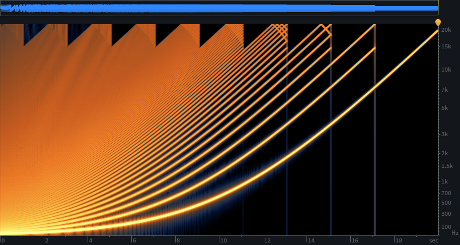
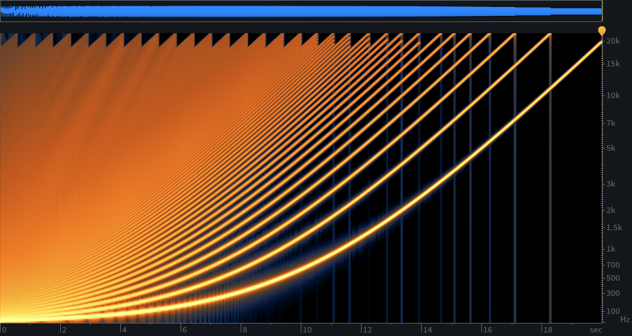
The catch is that our table of 2048 for 20 Hz doesn’t necessarily hold a sine wave. For a sawtooth, it holds harmonic 1001 with just over two samples. Linear interpolation fails miserably for producing that harmonic. The errors cause significant distortion and aliasing with that harmonic. And a whole lot of harmonics below it, but improving as we move towards the lower harmonics where they will be awesome.

Our first thought might be that we need a table size 128 times as large, to get up above 512 for the highest harmonic. So, 262,144 samples, just for the lowest table?

No, we cheat

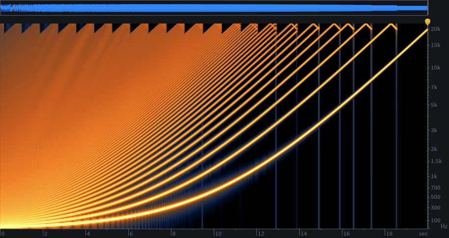
Here’s where psychoacoustics saves the day. Even though our distortion and noise floor figures for the higher harmonics look pretty grim, it’s extremely difficult to hear the problem over the sweetly rendered lower harmonics. And, fortunately, oscillators we like to listen to won’t likely have a weak fundamental and a strong extremely-high harmonic with nothing in between. Natural and pleasant sounding tones are heavily biased to the lower harmonics.

Also, if we choose to keep constant table sizes, then as we move up each octave, removing higher harmonics, the tables are progressively more oversampled as a result. Constant table sizes are convenient anyway, and don’t impact storage significantly. So, at the low end we’re saved by masking, and though we lose masking as we move up in frequency, at the same time the linear interpolation improves with increasingly oversampled tables. At the highest note we intend to play, near 20 kHz, error will be something like -140 dB relative to the signal.

Posted in Digital Audio, Oscillators, Wavetable Oscillators | 12 Comments

WaveUtils updated

WaveUtils needed only a minor change for compatibility with the WaveTableOsc update—addWaveTable changes to AddWaveTable. But I added something new while I was at it.

The original wave table articles advocated minimizing the number of tables necessary—one per octave—by allowing a reasonable amount of aliasing. Aliasing that is not only difficult to hear, but is normally be removed in typically synthesizer applications by the synth’s lowpass filter.

But that is simply a choice of the individual wave tables and how much of the spectrum we’re willing to let each cover. We could use more wave tables and allow no aliasing at all.

In addition to the fillTables function, which builds active wave tables. I’ve added fillTables2, which accepts a minimum top frequency, and a maximum top frequency. For instance, we might want to support a minimum of 18 kHz, using a value of 18000 divided by the sample rate, so that harmonics are supported to at least that frequency. If we use 0.5 for the maximum, then no aliasing is allowed. Higher values allow aliasing. For instance, a value of 0.6 allows a top frequency of 0.6 times the sample rate, or 26460 Hz at 44.1 kHz sampling. That’s 4410 above half the sample rate, so aliasing can extend down to 17640 Hz (22050 – 44100). Another way to look at it is to subtract the value from 1 and multiply by the sample rate to get the alias limit, (1 – 0.6) * 44100 = 17640.

Here are some examples. First, the original octave tables. To understand the spectrograms, time is left to right—a 20 second sweep from 20 Hz to 20 kHz of a sawtooth. You can see the aliasing as harmonic frequencies bend down at the top, although the algorithm minimizes the aliasing with advantageous choices of switching frequencies at the highest sweep frequencies, where there is the least masking. This uses ten wave tables to sweep the ten octaves of audio from 20 Hz to 20 kHz.

I think the aliasing is masked pretty well. But if the idea of aliasing bothers you, and you want at least 18 kHz coverage, 34 wave tables will get you this, at 44.1 kHz sample rate:

Now for an asymmetrical example. If you want 18 kHz, but are willing to accept aliasing above 20 kHz, 24 wave tables will do it:

WaveUtils source

Posted in Source Code, Wavetable Oscillators | 17 Comments

WaveTableOsc optimized

The wave table oscillator developed here in 2012 is pretty lightweight, but I never took a close look at optimization at the time. An efficient design is the number one optimization, and it already had that. I was curious how much minor code tweaks would help.

Free wrap

For instance, to avoid added complexity in the original article, I didn’t employ a common trick of extending the wave table an extra sample in order to avoid the need for a wrap-around test in the linear interpolation. A rewrite was a good opportunity to add it, and check on the improvement. The code change was trivial—add one to the allocation size for each table, and duplicate the first sample to the last when filling them, in AddWaveTable. Then remove the bounds check in the linear interpolation, saving a test and branch for every sample generated.

// old
float samp0 = waveTable->waveTable[intPart];
if (++intPart >= waveTable->waveTableLen)
    intPart = 0;
float samp1 = waveTable->waveTable[intPart];

// new
float samp0 = waveTable->waveTable[intPart];
float samp1 = waveTable->waveTable[intPart + 1];

Factor

And, I spotted another optimization opportunity. The oscillator needs to select the appropriate wavetable each time it calculates the next sample (GetOutput), but the choice of wavetable only changes when the frequency changes. So, the selection should be moved to SetFrequency. In general use, it should make no difference—an analog-like synth would usually have continuous modulation of the oscillator, for instance. But moving the calculation to SetFrequency would be a substantial win for steady tones.

I’ll go through the changes and their contributions, but a little explanation first. Unlike most of my DSP classes that provide a new sample on each Process call, the oscillator requires two calls—GetOutput and UpdatePhase—every time. It was just a design choice, I could have also provided a Process call that does both. In addition, SetFrequency might also be called every time, if the modulation is constant. For a steady tone, we’d call SetFrequency once, then the other two calls repeatedly for each sample. For a sweep, all three would be called for each sample. Of course I could trivially add a Process call that couples the existing UpdatePhase and GetOutput.

The wave table selection code iterates from lowest to highest, until it finds the right table, so it’s slower for higher frequencies. So, we’d expect an improvement in moving that code to SetFrequency for the steady tone case, and that the amount of improvement would be greater for high tone settings. We’d expect the case of a sweep to give no change in performance, since it still requires the wave table selection on each sample.

// old
inline void WaveTableOsc::setFrequency(double inc) {
  phaseInc = inc;
}

// new: the added code was simply repositioned from GetOutput
void SetFrequency(double inc) {
  mPhaseInc = inc;

  // update the current wave table selector
  int curWaveTable = 0;
  while ((mPhaseInc >= mWaveTables[curWaveTable].topFreq) && (curWaveTable < (mNumWaveTables - 1))) {
    ++curWaveTable;
  }
  mCurWaveTable = curWaveTable;
}

After moving the table selection from GetOutput, implementing the “one extra sample” optimization gave about a 20% improvement to the steady-tone case (SetFrequency not included) on its own. Unexpectedly, changing the variable temp from double to float gave a similar individual improvement. For steady tones, these changes together yielded a 30% improvement to the loop (SetFrequency not included), and 60% for high tones.

At first test, the sweep case did not see the improvement, as the biggest change simply moved the calculation between the two routines called on each sample. I was disappointed, because I expected at least a small improvement from the other changes, but instruction pipelines can be fickle. The minor tweak of using a temporary variable to calculate mCurWaveTable changed that—yielding a a 24% improvement. This is in a loop that sweeps a sawtooth exponentially through the audible range (SetFrequency, GetOutput, UpdatePhase, calculate the next frequency with a multiply, loop overhead). Basically, all the same code is executed, but apparently it worked out better for the processor. So, a great improvement overall.

Another goal of the change was to put everything in a single header file—because I like that. GetOutput was formerly not inline, so there was a small improvement moving it. I also changed the case of the function names (setFrequency to SetFrequency) to align with the way I currently write code, so it’s not a drop-in replacement for the old version.

I tried one other improvement. The wave table selection “while” loop takes longer, of course, as frequency moves to higher tables. I tried to special-case octave tables by using clever manipulation of a floating point number, essentially getting a cheap log conversion. The advantage would be a single calculation for any frequency, instead of an iterative search. It ended up not being worth it for the case of octave tables, the iterative solution was more efficient that I expected, and more importantly it’s far more general.

Using picobench to benchmark, the new code is about 25% faster for the case of a 20-20kHz sawtooth sweep. Not a huge change, because the code was already very efficient. But as part of single-header-file rewrite without increasing complexity, that’s a pretty good bonus.

WaveTableOsc.h

Posted in Source Code, Wavetable Oscillators | 6 Comments

How I write code

Next article I’ll post an update of our wave table oscillator, but first I’ll take the opportunity to discuss how I write code these days. Maybe it will help make sense of some of the choices in the code I post going forward.

I tend to build all DSP units as inlines in header files

True story: Recently, I moved an audio plug-in project I was developing on the Mac in Xcode, to Windows and Visual Studio. I was shocked to see that my source files had disappeared! There was only the main implementation cpp file (not counting the plugin framework), and my headers files. All files were backed up, of course, but it was still unsettling—what could have happened? Then it sank in—I’d written most of the good stuff in header files, so that outside of the plug-in framework, there was indeed only one cpp file—leveraging 28 header files.

The main reason my DSP functions reside in header files is that I make my basic functions inline-able for speed. In a perfectly orderly world, that still might be a header file for the smallest and most critical functions, and a companion C++ source file (.cpp) for the rest. But it’s faster to code and make changes to a single file instead of bouncing between two. And I need only include the header where I use it, instead of also pulling in and marking companion cpp files for compilation.

Further, I write “atomic” DSP components that handle basic functions, and build more complex components from these atomic functions. For instance, I have a delay line function, from which I make an allpass delay. Writing a reverb function can be very short and clear, combining these basic functions with other filter functions and feedback. And feedback is easy because all components process a sample at a time instead of blocks. Examples of my library files: OnePole.h, Biquad.h, StateVar.h, DelayLine.h, FIR.h, Noise.h, Gain.h, ADSR.h, WaveTableOsc.h.

Note that “inline” is a request to the compiler. But compilers are pretty good about honoring it. Remember, inline matters most for small functions, where function call overhead is a bigger consideration. And small functions are easiest to inline, so there’s little reason for a compiler to not comply. If you’re concerned, just list and examine the preprocessor output of a source file to see it.

By the way, the usual argument against inlines—“they lead to bloated code”—doesn’t apply much in the DSP context. These are not large functions used many places in your code. They are built for efficiency. The process routines are localized to your audio processing function, and the setting routines mostly in your plug-in’s parameter handling code.

My DSP units are designed for individual samples, not blocks of samples

Dedicated DSP chips usually process audio a sample at a time. But DSP run on a host computer’s process must handle audio a buffer at a time, to minimize the overhead of context switching. So, if you look at open source DSP libraries, you’ll see that many are written to operate on a buffer of samples.

I don’t do that—my inline functions process a single sample at a time. Of course, you can easily wrap that in a for loop, perhaps partially unrolled to minimize loop overhead. The the next process that acts on the entire buffer, then the next. Or you can string them together, one after the other, to complete your entire algorithm one sample at a time, with an outer loop to iterate through the buffer. The former might work better do the caching advantages, at the expense of more loop overhead. But it’s easier to make this choice with single-sample processes than for a library that’s entirely optimized for buffer processing.

I usually write my DSP units as templates

Mainly, I template them to handle float or double. I use double when developing, but have the option of float available. Filters are a case in which I’ll always use double. For a wavetable oscillator, I want double parameters but float wavetables. A delay line element might be float or double depending on the need. I’d rather build the choice into the DSP unit than to run into a different need and have to take time to rewrite the DSP unit or make a new version of it.

I tend to avoid posting templated stuff on my website, because it can be a distraction from what I’m trying to show.

No virtual functions

I don’t want a vtable. I’m not going to inherit from these basic DSP functions anyway, they are built to do one thing efficiently.

Minor detail: I wrap each DSP header file in a namespace. (I use namespace ESP—which stand for “EarLevel Signal Processing”.) Then I can be lazy with my class names without concern of one day having a namespace collision issue (my “Biquad” versus another “Biquad” built into the plug-in library, for instance).

Posted in Source Code | 18 Comments

Floating point denormals

There’s another issue with floating point hardware that can easily cause serious performance problems in DSP code. Fortunately, it’s also easy to guard against if you understand the issue. I covered this topic a few years ago in A note about de-normalization, but giving it a fresh visit as a companion to Floating point caveats.

Floating point hardware is optimized for maximum use of the mantissa, for best accuracy. (It also allows for more efficient math processing, since the mantissas are always aligned.) This is called normalization—all numbers are kept in the binary range of plus or minus 1.1111111 (keep going, 16 more 1s) times 2 raised to the power of the exponent. To increase accuracy near zero, floating point implementations let the number become “denormalized”, so instead of the smallest number being 1.0 times 2 raised to the most negative exponent, the mantissa can become as small as 0.000…1 (24 digits).

The penalty is that floating point math operations become considerably slower. The penalty depends on the processor, but certainly CPU use can grow significantly—in older processors, a modest DSP algorithm using denormals could completely lock up a computer.

But these extremely tiny values are of no use in audio, so we can avoid using them, right? Not so easily—recursive algorithms such as IIR lowpass filters can decay into near-zero numbers in typical use, so they will happen. For instance, when you hit Stop on your DAW’s transport, it likely sends a stream of zeros (to let reverbs decay out, and any live input through effects to continue). The memory of a lowpass filter then decays exponentially towards zero. We can slow it a bit by using double precision floats, but it’s only a matter of time till the processing meter climbs abruptly when your processing algorithm bogs down in denormalized computation.

Modern processors can mitigate the problem with flush-to-zero and denormals-are-zero modes. But this too can be tricky—you’re sharing the processor with other functions that might fail without the expected denormal behavior. You could flip the switch off and back during your main DSP routine, but you need to be careful that you’re not calling a math function that might fail. Also, this fix is processor dependent, and might be the wrong thing to do if you move your code ot a new platform. A DSP framework might handle this conveniently for you, but my goal here is to show you that it’s pretty easy to work around, even without help from the processor. Let’s look at what else we could do.

We could test the output of any susceptible math operation—there is no need to test all operations, because most won’t create a denormal without a denormal as input.

There’s a surprisingly easy solution, though, and it’s more efficient than testing and handling each susceptible operation. At points that have the threat of falling into denormals, we can add a tiny value to ensure it can’t get near zero. This value can be so small that it’s hundreds of dB down from the audio level, but it’s still large compared with a denormal.

In fact, it’s actually possible to flush denormals to zero with no other error, due to the same properties of floating point we discussed earlier. If you add a relatively large number to a denormal, then subtract it back out, the result is zero. Still, this is pointless, because a tiny offset will not be heard.

But there is a catch to watch out for. A constant value in the signal path is the same as a DC offset. Some components, such as a highpass filter, remove DC offsets. I get around this by using a tiny number to add as need in the signal path—often, one time is enough for an entire plugin channel—and alternating the sign of it each time a new buffer is processed. A value such as 1e-15 (-300 dB) completely wipes out denormals while having no audible effect.

Why did I pick that value? It needs to be at least the smallest normalized number (2^-126, about 1e-38, or about -760 dB), to ensure it wipes out the smallest denormal. That would work, but it’s better to use a larger number so that you don’t have to add it in as often. A much larger number would likely be fine to add just once—just add it to the input sample, for instance. (But consider your algorithm—if you have a noise gate internal to your effect, you might need to add the the “fixer” value after its output as well.) And clearly it needs to be small enough that it won’t be heard, and won’t affect algorithms such as spectrum analysis. A number like 1e-15 is -300 dB—each additional decimal place is -20 dB, so 1e-20 is -400 dB, for instance. Let your own degree of paranoia dictate the value, but numbers in those ranges are unlikely to affect DSP algorithms, while wiping out any chance of denormals through the chain.

To recap: Take a small number (mDenormGuard = 1e-15;). Change its sign (mDenormGuard = -mDenormGuard;) once in a while so a DC blocker you might have in your code doesn’t remove it. A handy place is the beginning of your audio buffer handling routine, one sign change for an entire buffer should be fine. Add it in (input + mDenormGuard).

Here’s an example of my plug-in (Amp Farm native), during development, showing the performance meter in a DAW while processing audio:

With denormal protection turned off, the performance is the same while processing normal audio, but a few seconds after stopping the transport, the load rises due to denormals:

With denormal protection enabled, performance looks like the first picture at all times. And that’s why we protect against denormals!

Posted in Math | 10 Comments

Floating point caveats

The equivalent of “When I was your age, we use to walk to school in the snow. Barefoot”, in DSP, is to say we used to do DSP in fixed point math. The fixed-point system could be made of integer and shift operations in software, or built into fixed-point DSP chips such as the 56K family, or other hardware implementations. Floating point was not available in dedicated DSP chips, and took too many cycles on a CPU. But the general usefulness of floating point lead to it being optimized in CPUs, making it the overwhelming choice for DSP today.

A floating binary point allows floating point math a huge range. It essentially gives us a magic ruler that can be stretch or shrunk at will, to measure huge or tiny distances with the same relative accuracy. The catch is the word “relative”. There are the same number of tick marks on the ruler at any size, and that makes for some properties that might not be immediately obvious. Besides the effects of math involving quantized samples, significant errors to watch out for are in addition, multiplication, and denormals. We’ll cover denormals in the next post.

Definitions

Floating point is well defined in IEEE standards that are widely adopted in order to give consistent results from one computer and processor to another. There are many ways to do floating point, but these are the only ones we need consider.

“Single precision” (32-bit) floating point, “float” in C, is ample to hold samples of a digital audio stream. It has a sign bit, 23 bits of mantissa, and 8 bits of exponent. But floating point execution units typically keep results in a “normalized” state, where the leading digit is always a “1” and the exponent is adjusted accordingly. This makes best use of the available mantissa bits. Since the leading bit is always 1, it’s omitted, yielding 24 mantissa bits, effectively. But we have a sign bit too, so it’s equivalent to 25-bit audio. It matches up conveniently to 24-bit audio converters.

Double precision (64-bit), “double” in C, gives substantially more of everything, at little cost in processing time (though twice the memory use). A sign bit, 52 bits of mantissa, and 11 bits of exponent. The increase in exponent isn’t important for audio, but the 54 bits of precision is a big plus to minimize accumulated errors.

For an idea of how the two compare, precision-wise, consider that there are 31557600 seconds in a year. The 25 bits of effective precision (if using the full range of negative to positive) in a 32-bit float has a range of 33554432 (225), a resolution of about a second out of a year. A 64-bit double has a range of 18014398509482000 (254), for a resolution of about two nanoseconds.

For fixed point, it depends on the implementation but the standard is the 56k family, which multiplies 24-bit (leading decimal point) numbers for a result with 48 bits to the right of the decimal point and 8 to the left. The extra 8 bits allow headroom for multiply-accumulate cycles to grow greater than one.

Which size to use

32-bit floats are ample for storage and for the sample busses between processing—the 64-bit sample size used for buffers by some DAWs is overkill. 32-bit floats are adequate for many computations, on par with 24-bit fixed point systems (better in most regards but falling short in some—the 56K’s extended-precision accumulators allow long FIRs to be more precise). Either size has far more range in the exponent than we’ll use—audio simply doesn’t require that incredible dynamic range.

But CPUs are heavily optimized for double-precision floating point, and the added precision is often necessary in audio DSP algorithms. For typical modern Mac/PC host processors, stick with doubles in your DSP calculations; the performance difference is small, and your life will be a lot easier, with less chance of a surprise. But you may need to use single-precision, especially in DSP chips or SIMD and some processors where the performance difference is large, so you should understand the limitations.

Errors in multiplication

When you multiply two arbitrary numbers of n digits of precision, the result has 2n digits of precision. 9 x 9 = 81, 99 x 99 = 9801, .9 x .9 = .81. But floating point processors do not give results in a higher precision—the result is truncated to fit in the same number of bits as the operands (essentially, .1111 x .9999 = .1110 instead of the precise .11108889, for an example of 4-digit decimal math). This means an algorithm using single precision floats may have significantly more error than the same algorithm done in a fixed point DSP like the 56K family, which allows accumulation of double-precision results. You need to consider the effects of this error on your algorithm. Or, just stick with double precision computation, which has so much precision that you can usually ignore this truncation error for audio (but watch out for things like raising values to high powers—you can’t freely code arbitrarily high-order IIR filters even with doubles, which is why we usually factor higher orders into a cascade of biquads).

Errors in addition

If you’ve worked with fixed-point math, you’re used to the idea that you discard precision from multiplying when storing back to the original sample size, but addition is basically perfect (as long as you don’t overflow, by either guarding against it, or using an accumulator with headroom). With floating point, you have the same fundamental issues as with multiplication (but with no choice), and a whole new problem with addition. I think this is something many don’t consider, so this section might be my most important point.

Floating point doesn’t do well when adding two values of vastly different sizes.

If our magic ruler is stretched to measure the distance from here to the sun, each tick is bout 5 km, so adding a measurement of a bug’s wing to it will do nothing—it’s too small of a distance to make it to the next tick, the next highest possible number. (With zero placed at the midpoint of the span, the effective mantissa range of a 32-bit float is 225, or 33554432. The scale is our distance to the sun, 150 million km—150000000 km / 33554432 is about 5 km per “tick”. For doubles, it’s half the width of the finest human hair!)

This can be a huge problem in iterative math. Consider that a 32-bit unsigned integer has a maximum value of 4,294,967,295. As long as you don’t exceed that amount, you can count through every value from 0 to that maximum by adding one for each count. A 32-bit float has a maximum value of 3.402823 × 1038, but can count through a maximum of 16,777,216 steps incrementally, no matter the size. After that, the increment is too small compared with the size of the running total, and has no effect.

For instance, a big mistake would be to use a 32-bit float as a timer, incrementing every sample period, to use in an automation ramp calculation. Even if the time increment is a very small number, the timer will stop incrementing after six minutes because the increment’s mantissa can no longer be aligned with that of the running total. 6.3 minutes * 60 seconds/minute * 44100 samples/second is about 224 (16777216) samples—we’re assuming only positive values here. The good news is that when using doubles, it would take a few thousand years to hit that point.

Try this:

// Incrementing integer and float
#include <iostream>
#include <cstdint>
using namespace std;

int main() {
    const long objectives[] = { 100, 10000, 1000000, 100000000, 1000000000 };
    for(const long objective : objectives) {
        float counterFp = 0;
        uint32_t counterInt = 0;
        for (long idx = 0; idx < objective; idx ++) {
            counterInt += 1;
            counterFp += 1;
        }
        cout.precision(20);
        cout << counterInt << ",  " << counterFp << endl;
    }
}
100,  100
10000,  10000
1000000,  1000000
100000000,  16777216
1000000000,  16777216

Note that fixed point math is not without this problem, but for fixed point it’s obvious that small numbers use fewer significants after the leading zeros, and obvious when they are too small to fit in the fixed point representation. With floating point, you can be easily fooled into thinking you have more precision in a value than you can use for an addition operation, because the usable precision is dependent on the value you’re adding it to.

Posted in Math | 9 Comments

Wavetable signal to noise ratio

In our wavetable series, we discussed what size our wavetables needed to be in order to give us an appropriate number of harmonics. But since we interpolated between adjacent table entries, the table size also dictates the signal to noise ratio of playback. A bigger (and therefore more oversampled) table will give lower interpolation error—less noise. We use “signal to noise ratio”—SNR for short—as our metric for audio.

SNR has a precise definition—it’s the RMS value of the signal divided by the RMS value of the noise, and we usually express the ratio in dB. We’ll confine this article to sine tables, because they are useful and the ear is relatively sensitive to the purity of a sine wave.

We could derive the relationship of table size and SNR analytically, but this article is about measurement, and it’s easily extended to other types of waveforms and audio.

Calculating SNR

To calculate SNR, we need to know what part of the sampled audio is signal and what part is noise. Since we’re generating the audio, it’s pretty easy to know each. For example, if we interpolate our audio from a sine table, the signal part is the best precision sine calculations we can make, and the noise is that minus the wavetable-interpolated version. RMS is root-mean-squared, or taking the square roots of all the samples, producing the average, then squaring that value. We do that for both the signal and the noise, sample by sample, and divide the two—and convert to dB. The greatest error between the samples will be somewhere in the middle. Picking halfway for the sine is a good guess, but we can easily take more measurements and see.

It ends up that the table size can be relative small for an excellent SNR with linear interpolation. This shouldn’t be surprising, since a sine wave is smooth and therefore the error of drawing a line between two points gets small quickly with table size. A 512 sample table is ample for direct use in audio. It yields a 97 dB SNR. While some might think that’s fine for 16-bit audio but not so impressive for 24 bit, a closer look reveals just how good that SNR is.

Keep in mind, this is a ratio of signal to noise. While the noise floor is -97 dB compared with the signal, that’s not the same as saying we have a noise floor of -97 dB. The noise floor is -97 dB when the signal is 0 dB (actually, this is RMS, so a full-code sine wave is -3 dB and the noise is -100 dB). But people don’t record and listen to sine waves at the loudest possible volume. When the signal is -30 dB, the noise floor is -127 dB. When the signal is disabled, the noise floor is non-existent.

However, if that’s still not good enough for you, every doubling of the table size yields a 20 dB improvement.

Code

Here’s a simple C++ example that calculates the SNR of a sine table. Set the tableSize variable to check different table sizes (typically a power of 2, but not enforced). The span variable is the number of measurements from one table entry to the next. You can copy and paste, and execute, this code in an online compiler (search for “execute c++ online” for many options).

#include <iostream>
#include <cmath>
#if !defined M_PI
const double M_PI = 3.14159265358979323846;
#endif
using namespace std;

int main(void) {
    const long tableSize = 512;
    const long span = 4;
    const long len = tableSize * span;
    double sigPower = 0;
    double errPower = 0;
    for (long idx = 0; idx < len; idx++) {		
        long idxMod = fmod(idx, span);

        double sig = sin((double)idx / len * 2 * M_PI);

        double sin0, sin1;
        if (!idxMod) {
            sin0 = sig;
            sin1 = sin((double)(idx + span) / len * 2 * M_PI);
        }

        double err = (sin1 - sin0) * idxMod / span + sin0 - sig;

        sigPower += sig * sig;
        errPower += err * err;
    }
    sigPower = sqrt(sigPower / len);
    errPower = sqrt(errPower / len);

    cout << "Table size: " << tableSize << endl;
    cout << "Signal: " << 20 * log10(sigPower) << " dB RMS" << endl;
    cout << "Noise:  " << 20 * log10(errPower) << " dB RMS" << endl;
    cout << "SNR:    " << 20 * log10(sigPower / errPower) << " dB RMS" << endl;
}

Quantifying the benefit of interpolation

This is a good opportunity to explore what linear interpolation buys us. Just change the error calculation line to “double err = sin0 – sig;”, and set span to a larger number, like 32, to get more readings between samples. Without linear interpolation, the SNR of a 512-sample table is about 43 dB, down from 97 dB, and we gain only 6 dB per table doubling.

You can extend this comparison to other interpolation methods, but it’s clear that linear interpolation is sufficient for a sine table.

Extending to other waveforms

OK, how about other waveforms? A sawtooth wave is not as smooth as a sine, so as you might expect, it will take a larger table to yield high SNR number. Looking at it another way, the sawtooth is made up of a sine fundamental. The next harmonic is at half the amplitude, which alone would contribute half the signal and half the noise, but it’s also double the frequency—the equivalent of half the sine table size and therefore 20 dB worse than the fundamental is taken alone. It’s a little more complicated than just summing up the errors of the component sines, though, because positive and negative errors can cancel.

But the measurement technique is basically the same as with the sine example. The signal would be a high-resolution bandlimited sawtooth (not a naive sawtooth), and noise would be the difference between that and the interpolated values from your bandlimited sawtooth table. Left to you as an exercise, but you may be surprised at the poor numbers of a 2048 or 4096 sample table in the low octaves (where the is no oversampling). But again, the noise only occurs when you have signal, particularly when you have a bright waveform, and remains that far below it at any amplitude. It’s still hard to hear the noise through the signal!

Checking the SNR of wavetable generated by our wavetable oscillator code is a straightforward extension of the sine table code. For a wavetable of size 2048 and a given number of harmonics, for instance, create a table of size 2048 times span. Then subtract each entry of the wavetable, our “signal”, from the corresponding interpolated value for the “noise”. For instance, if tableSize is 2048 and span is 8, create a table of 16384 samples. For each signal sample n, from 0 to 16383, compare it with the linearly interpolated value between span points (compare samples 0-7 with the corresponding linear interpolation of samples 0 and 8, etc., using modulo or counters).

It’s more code than I want to put up in this article, especially if I want to give a lot of options or waves and interpolations, but it’s easy. You might want to make a class that lets you specify a waveform, including number of harmonics and wavetable size, which creates the waveform. Create a function to do the linear interpolation (“lerp”) and possibly others (make it a class in that case); input the wavetable and span, output the computed signal and noise numbers. Then main simply makes the call to build the waveform, and another call to analyze it, and displays the results.

Posted in Digital Audio, Oscillators, Wavetable Oscillators | 2 Comments

Sampling theory, the best explanation you’ve ever heard—End notes

A few words before moving on to other topics…

We’ve looked at why digital sample represent ideal impulses, and why any point between samples represents a value of zero. And, as a result, audio samples don’t represent the audio itself, but a modulated version of the audio.

Why is helpful to understand these points?

Critical sampling

First, it gives clear and intuitive answers for why digital audio behaves certain ways than do more typical explanations. For instance, it makes this puzzle trivial:

People ask why the sample rate needs to be double the frequency of the highest signal frequency that we want to preserve. Often the reply is that it needs to be just above double the highest frequency of interest, to avoid aliasing. But why? And how much higher? At this point, someone mentions something about wagon wheels turning the wrong way in movies. Or shows a graph with two sine waves of different frequencies intersecting the same sample points. So unsatisfying.

If you consider that the signal is amplitude modulated in the digitization process, you need only see that the sidebands would start overlapping at exactly half the sample rate. To keep them from overlapping, all frequencies must be below half the sample rate, giving each cycle more than two samples.

Multistage conversion

And integer sample rate conversion choices are easier to make. Especially for multistage conversion. We often use multistage conversion to improve efficiency. Like performing 8x upsampling as three 2x stages. If that sounds like three times the work, it isn’t, because the higher relative cutoffs of the filters make for fewer coefficients, balancing out with the total operations for 8x. But we can do more than break even by optimizing each stage—the earlier stages can be a bit sloppy as long as everything is tidy by the last stage’s output. Somewhat like doing a big cleanup on a house in multiple passes versus one.

Perhaps this is a good place to note that you might see chatroom posts where someone says that instead of inserting zeros and filtering, they prefer to use a polyphase filter. There is no difference—a polyphase filter in this case is simply an algorithm that upsamples and filters. Any seasoned programmer will notice that there is no need to explicitly place zeros between samples, then run all samples through an FIR, because the zero samples result in a zero product; optimizing the code to skip the zero operations results in a polyphase filter.

Optimization example

An understanding of why we need to filter rate conversions can help us optimize DSP processes. For example, someone posted a question on a DSP board recently. They were using EQ filters designed by the bilinear transform, which have a pinching effect near half the sample rate (due to zeros at the Nyquist frequency). They didn’t need additional frequency headroom per se—the filters are linear—but they wanted to oversample by 2x to avoid the shape distortion of peaking EQ filters. (Note there are methods to reduce or avoid such distortion of the filter shape, but this is a good example.)

Let’s say we’re using a 48 kHz sample rate. Typically we’d raise the sample rate to 96k by inserting zeros every other sample and then lowpass filtering below 24k. Then we’d do our processing (EQ filtering). Finally, we’d take it back to 48k by lowpass filtering below 24k and discarding every other sample. But in this case, our processing step is linear (linear EQ filters), so it doesn’t create new frequencies. That means we can skip one of the lowpass filtering stages. It doesn’t matter whether we lowpass filter before or after the EQ processing, but we don’t need both. That’s a substantial savings.

Another example

Let’s say we create an audio effect such as an amp simulator, which has a non-linear process that requires running at a higher sample rate to reduce audible aliasing. We run our initial linear processes, such as tone controls, then upsample and run our non-linear processes (an overdriven tube simulation!). But in this case we conclude with a speaker cabinet simulator, which is a linear process (via convolution or other type of filtering). Guitar and bass cabinets use large speakers (typically 8” and up, often 10” or 12” for guitar), with frequency responses that drops steeply above around 5 kHz. Understanding how the downsampling process works, we might choose to eliminate the downsampling filter stage altogether, as superfluous, or at least save cycles with a simplified filter with relaxed requirements.

Posted in Digital Audio, Sampling Theory | Tagged | 2 Comments

Sampling theory, the best explanation you’ve ever heard—Part 3

We look at what Pulse Amplitude Modulation added to our analog source audio.

What did PAM add?

Earlier, we noted that the PAM signal represents the the source signal plus some additional high frequency content that we need to remove with a lowpass filter before we listen back.

Again, PAM is amplitude modulation of the source signal with a pulse train. Mathematically, we know precisely what amplitude modulation produces—the sums and differences of every frequency component between the two input signals. That is, if you you multiply a 100 Hz sine wave by a 6 Hz sine wave, the result is the sum of 106 Hz and 94 Hz sine waves. For signals with more frequency components, there are more sums and differences in the result.

To answer our question, “What got added?”, we need to understand the frequency content of a pulse train. One way to know that would be to use an Fourier Transform on the pulse train. But I want to use intuitive reasoning to eliminate as much math as possible. Fortunately, I already know what the extra frequency content is—it’s the spectral images in sampled systems, as described in classic DSP textbooks. That coupled with knowledge of amplitude modulation tips me off that we’ll need a frequency component at 0 Hz (DC—we need that to keep our original source band), at the sample rate, and at every integer multiple of the sample rate. Through infinity.

OK, we’ll lighten up on the infinity requirement. We can’t produce a perfect impulse in the analog world anyway. And we don’t need to. However, once in the digital domain, samples represent perfect impulses. While their values may have deviated slightly from a perfect representation of the analog signal, due to sampling time jitter and quantization, any math we do to them is “perfect” (again, subject to quantization and any other approximations). In the digital realm, the images do go to infinity.

Indeed, as you add cosine waves of 0, 1, 2, 3, 4…times the sample rate, the result gets closer and closer to the shape of an impulse. (Cosine instead of sine so that the peaks of the different frequencies line up.)

And that means we’ll have a copy of the source signal mirrored around 0 Hz, around the sample rate, twice the sample rate, three times the sample rate…to infinity. (In both directions, but we can ignore negative frequencies—for real signals, the negative spectrum mirrors the positive.)

What we’ve learned

Revisiting my “secrets”, with added comments:

1. Individual digital samples are impulses. Not bandlimited impulses, ideal ones.

Bothered that ideal impulses are impossible? Only in the physical world. There, we accept limitations. For instance, gather together infinity of something. Anything—I’ll wait. Meanwhile, in the mathematical world, infinity fits easily on this page: ∞

2. We know what lies between samples—virtual zero samples.

Think there’s really a continuous wave, implied, between samples? If so, you probably think it’s because samples represent a bandlimited impulse. No—you’re getting confused with what will come out of the DAC’s lowpass filter later, when we play back audio.

3. Audio samples don’t represent the source audio. They represent a modulated version of the audio. We modulated the audio to ensure points #1 and #2.

This is a frequency-domain observation that follows from the first two points, which are time domain. If you understand this point, you’ll never be confused about sample rate conversion.

Posted in Digital Audio, Sampling Theory | Tagged | 5 Comments

Sampling theory, the best explanation you’ve ever heard—Part 2

In this article, we explore the origins of sampling.

Discrete time

For many, discrete time and digital sampling are synonymous, because most people have little experience with discrete time analog. But perhaps you’ve used an old-style analog delay stompbox, with “bucket brigade” delay chips. Discrete time goes back a lot farther, though. When we talk of the sampling theorem, attributed to people like Nyquist, Shannon, and others, it applies to discrete time signals, not digital signals in particular.

The origins of discrete time theory are in communications. A single wire can support multiple simultaneous telegraph messages, if you synchronize a commutator between sender and receiver and slice time into sections to interleave the messages—this is called Time Division Multiplexing, or TDM. Following later with voice, using TDM to fit multiple voice calls on a line, it was found that the sampling rate had to be around 3500-4300 Hz for satisfactory results.

Traveling over a wire, analog signals can’t be “discrete” per se–there is always something being sent, no gaps in time. But the signal information is discrete, sending zero in between, and that leaves room to interleave other signals in TDM.

The most common method of making an analog signal discrete in this way is through Pulse Amplitude Modulation, or PAM. This means we multiply the source signal continuously with a pulse train of unit amplitude.

While the benefit of PAM for analog communications is that we can interleave multiple signals, for digital, the benefit is that we don’t need to store the “blank” (zero) space between samples. For digital sampling, we simply measure the height of each impulse of the PAM result, and encode it as a number. Pulse Amplitude Modulation and encoding—we call the combined process Pulse Code Modulation. Now you know what PCM means.

Impulses, really

Some might look at that last diagram and think, “But I’ve seen this process depicted as a staircase wave before, not spiky impulses.” In fact, measuring voltage quickly and with precision, which we must do for the encoding step, is not easy. Fortunately, we intend to discard the PAM waveform anyway, and keep just the digital values. We don’t need to maintain the empty spaces between impulses, since our objective is not time division multiplexing analog signals. So, we perform a “sample and hold” process on the source signal, which charges a capacitor at the moment of sampling and stretches the voltage value out, allowing a more leisurely measurement.

This results only in a small shift in time, functionally identical to instantaneous sampling—digital samples represent impulses, not a staircase. If you have a sample value of 0.73, think of it as an impulse of height 0.73 units.

The step of digitizing the analog PAM signal introduces quantization, and therefore quantization error. But it’s important to understand that issues related to aliasing are not a property of the digital domain—aliasing is a property of discrete time systems, so is inherent in the analog PAM signal as well. That’s why we took this detour—I believe I can explain aliasing to you in a simpler way, from the analog perspective.

Next: We’ll look at exactly what frequency content is added by the PAM (and therefore PCM) process, in Part 3

Posted in Digital Audio, Sampling Theory | Tagged | Leave a comment