In a previous article, we looked at sample rate conversion in the frequency domain. Let’s take a quick second look in the time domain as reinforcement of principles behind sample rate conversion, before developing a practical rate convertor.
In an ideal digital to analog convertor, we output a pulse train in which each pulse’s amplitude corresponds to a sample value. The pulse train is processed by a lowpass “reconstruction” filter, to arrive at our smooth analog signal output. Theoretically, we want a perfect impulse into a perfect “brick wall” lowpass filter—one with no phase shift.
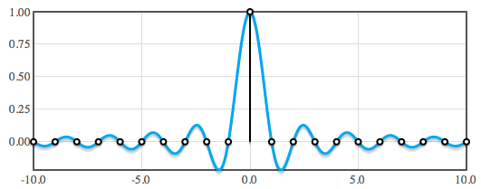
A perfect impulse into our perfect lowpass filter would give an output response of the sinc function; here is the “normalized” sinc function:
sin (π * x) / (π * x) { or 1, for x = 0 }
Here’s what it looks like, as does the output of our perfect filter when pinged by a perfect unit impulse (the curve tails off infinitely in both directions):
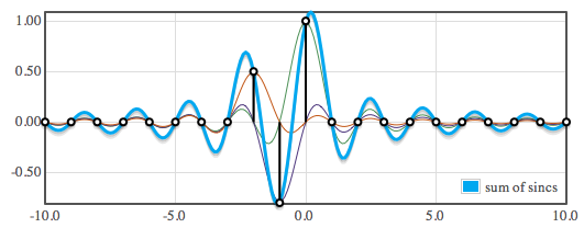
When we feed the filter with our impulse train, representing output samples, the individually responses for each impulse add together to make the analog output waveform. Here’s an example with three non-zero samples:
From this it should be apparent how to convert samples rates—sum those individual impulse responses for every new point that you need to determine. For instance, if you want to double the sample rate, simply calculate the points on that curve that are half-way between existing samples.
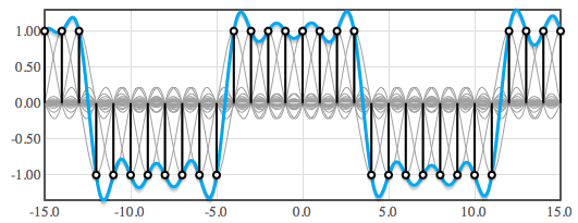
Need further convincing? Before moving on, let’s take a look at a digital square wave (-1,-1,-1,-1,+1,+1,+1,+1…), and sum the individual sinc impulse responses:
You probably recognize that as the look of a bandlimited square wave, so it looks like we’re on the right track.
Making it practical
The problem with our filter is in its perfection. Even if we could make this ideal filter from real-world components, we would wait forever for the output—the output would build slowly for an infinite amount of time until it peaked at a height corresponding to the input impulse, then die out over an infinite amount of time.
Fortunately, the sinc function gets smaller and smaller in each direction. We could let it run in both directions until the “lobes” got so small that they wouldn’t contribute to the quantized output, and truncate it from there. That’s still a long ways, which translates into a lot of output delay and a lot of calculations for the task we’re building up to. Fortunately, since the lobes are getting smaller and smaller, we can make a rough approximation by hastening their retreat with a window function that tapers the curve quicker. (Tapering gives better results than simply chopping off the ends—a rectangular window.)
Luckily for us, the difference between ideal and our tapered approximation is small, error-wise. This shouldn’t be surprising, since we know that real-world lowpass filters are far from perfect in cutoff slope, yet we find them very useful and audibly pleasing.
In addition to scaling the sinc function with the window, this is a good time to normalize the function for unity gain. The DC gain of the filter is the sum of the coefficients—this is true of any FIR filter. (This should be apparent, if you consider the output for the case of all input samples being 1.0.) The gain will vary depending on the filter settings, and be pretty close to the inverse of the factor used to calculate the sinc (for a filter with cutoff set to half the audio band, it will be about two, for instance). We simply divide each coefficient by the sum of the coefficients to achieve unity gain.
Putting the pieces together
Before continuing, here are some observations to keep in mind:
1) We chose the sinc function because it is the impulse response of a lowpass filter with an infinitely steep slope at cutoff (“brick wall”), and linear phase. (We may not always require linear phase, but in the general case, that’s what we want.)
2) We use a window function to convert our ideal filter into a practical one. It’s not the only way. We could trade off errors in a different way (the Park-McClellan algorithm, for instance). This article uses a windowed-sinc function because it’s a popular choice, and is easy to understand and implement.
There are many popular choices for window functions. Any of them give better results than simply truncating the sinc curve. The Kaiser window is an excellent choice for audio; it’s more complicated to calculate than most, but has the advantage of being able to set the level of tradeoff between stopband attenuation and sharpness of the cutoff easily. The cutoff steepness is dictated mainly by the number of side-lobes of the sinc response that we keep, hence the length of the filter. And because we’ve deviated from the perfect filter, we’ll need to set the cutoff below the ideal.
Here is what our normalized windowed sinc looks like, along with its components:
Coming next
Next up, we’ll have a have a windowed-sinc calculator that will help us compute coefficients for a high-quality sample rate convertor.


where is the previous part of this article ? no arrow/link obvious.
the diagram shows a square wave being recreated
but not the original one
looks like several db loss due to A/D D/A chain
this is okay if all you want is the shape of the signal
which you can amplify to get the original
or amplify more to play on loudspeakers
how does one know what the db loss was
for those who do need the original signal ?
I’ve redesigned the site in the past couple of weeks, upgrading from the entirely hand-coded html from 1996 (finally!). In some older articles, I’ve linked directly to other articles referenced, but I’m thinking I should add the references in a section after the article instead, still sorting this out—thanks for the comment.
The square wave is shown just as a point of reference. In the first example, with three impulses, the individual contributions can be seen easily, but it’s not intuitively obvious that the result is correct. Most people who’ve gotten this far are familiar with what a bandlimited square wave looks like, so I included it for that reason. It’s shown as unit impulses for convenience, but in practical terms it could have only been generated computationally (say, from a synthesizer). It’s very unlikely that you would get this from sampling with an A/D.
As far as dB in the general sense, the process is always relative—nothing absolute is recorded. You need a calibrated system to get out exactly what you put in. Of course, I’m addressing digital audio here, where it’s a non-issue—we scale from the singer to the mic to the preamp to the mixer to the A/D to the processing to the D/A to the amp to the speakers…
I do appreciate your comments—good to know someone’s reading!
“In addition to scaling the sinc function with the window, this is a good time to normalize the function for unity gain. The DC gain of the filter is the sum of the coefficients—this is true of any FIR filter. (This should be apparent, if you consider the output for the case of all input samples being 1.0.) The gain will vary depending on the filter settings, and be pretty close to the inverse of the factor used to calculate the sinc (for a filter with cutoff set to half the audio band, it will be about two, for instance). We simply divide each coefficient by the sum of the coefficients to achieve unity gain.”
There must be a trick to it. I am doing gross up-sampling (400x or more). When I sum the coefficients of my filter, I get a number in the thousands. If I normalize that way the output of the convolution disappears. My filter is generated thus:
K = 2.0 * PI * cutoff / rate
For FilterIndex As Integer = 0 To numTaps / 2
x = (FilterIndex – (numTaps / 2)) * K
If x = 0 Then
Sinc = 1.0
Else
Sinc = Sin(x) / x
End If
taps(FilterIndex) = Sinc
FilterTaps(numTaps – FilterIndex) = Sinc
Next FilterIndex
The cutoff frequency is 100 Hz, the sample rate is 1 megasample/sec. NumTaps is typically 75000. Obviously I’m not doing this in real time.
Any suggestions?
A quick look, but your sinc function looks fine, and yes, I’d expect a gain in the thousands. (Of course, I’d window the sinc, but maybe you’re giving this a rough try.) You should be able to sum the coefficients up, then divide each coefficient by that value. Make sure you have the convolution right. Doing that rate conversion in a single pass means that you’re stuffing a lot of zeros (or, more efficiently, doing the same thing with something resembling a polyphase filter).
I suggest making your software general enough, if it isn’t already, that you can test it with a smaller ratio (2x, for instance), and take a look at your input signal, coefficients, and output. If you can spit them out into a text file of numbers separated by commas, with a “.csv” extension, you can open it in a spread sheet and plot it (if you don’t already have something better). An impulse (a 1.0 followed by zeros) is a good choice for input to test your convolution, since the output should still look like the sinc function when you graph it.
what trips me out is that analog output of a digital impulse (1 followed by 00’s) has that pre ripple or ringing. almost like its backward in time? is that related to the whole gibbs thing?
I think that’s unsettling for many people the first time they think about it. There are a number of ways you can look at it, but to be brief, an impulse is the result of all frequencies at the same magnitude, energies centered on one point in time. So, if you strip away higher frequencies that sharpen the response, the remainder will spread out symmetrically. Of course, the part that makes it confusing is that it doesn’t happen in the real world. For instance, if we slap our hands together sharply, then repeat with a barrier to muffle the sound, the sound is not delayed with pre-ringing. That’s because filters in the real world can’t be linear phase—the energy is still focused at the time of the slap, and the ringing gets spread out after. And we’d get the same thing in the digital processing world if we used a minimum phase filter. The bottom line is that a linear phase filter is a math construct that uses time delay to maintain the phase relationships of component frequencies.
^ This is an utterly satisfaying and convincing answer, one that I wish my teachers had given me at the very beginning of my studies. Thank you