In this article, we explore the origins of sampling.
Discrete time
For many, discrete time and digital sampling are synonymous, because most people have little experience with discrete time analog. But perhaps you’ve used an old-style analog delay stompbox, with “bucket brigade” delay chips. Discrete time goes back a lot farther, though. When we talk of the sampling theorem, attributed to people like Nyquist, Shannon, and others, it applies to discrete time signals, not digital signals in particular.
The origins of discrete time theory are in communications. A single wire can support multiple simultaneous telegraph messages, if you synchronize a commutator between sender and receiver and slice time into sections to interleave the messages—this is called Time Division Multiplexing, or TDM. Following later with voice, using TDM to fit multiple voice calls on a line, it was found that the sampling rate had to be around 3500-4300 Hz for satisfactory results.
Traveling over a wire, analog signals can’t be “discrete” per se–there is always something being sent, no gaps in time. But the signal information is discrete, sending zero in between, and that leaves room to interleave other signals in TDM.

The most common method of making an analog signal discrete in this way is through Pulse Amplitude Modulation, or PAM. This means we multiply the source signal continuously with a pulse train of unit amplitude.
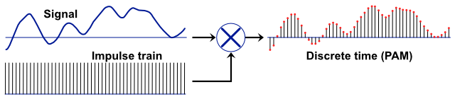
While the benefit of PAM for analog communications is that we can interleave multiple signals, for digital, the benefit is that we don’t need to store the “blank” (zero) space between samples. For digital sampling, we simply measure the height of each impulse of the PAM result, and encode it as a number. Pulse Amplitude Modulation and encoding—we call the combined process Pulse Code Modulation. Now you know what PCM means.
Impulses, really
Some might look at that last diagram and think, “But I’ve seen this process depicted as a staircase wave before, not spiky impulses.” In fact, measuring voltage quickly and with precision, which we must do for the encoding step, is not easy. Fortunately, we intend to discard the PAM waveform anyway, and keep just the digital values. We don’t need to maintain the empty spaces between impulses, since our objective is not time division multiplexing analog signals. So, we perform a “sample and hold” process on the source signal, which charges a capacitor at the moment of sampling and stretches the voltage value out, allowing a more leisurely measurement.

This results only in a small shift in time, functionally identical to instantaneous sampling—digital samples represent impulses, not a staircase. If you have a sample value of 0.73, think of it as an impulse of height 0.73 units.
The step of digitizing the analog PAM signal introduces quantization, and therefore quantization error. But it’s important to understand that issues related to aliasing are not a property of the digital domain—aliasing is a property of discrete time systems, so is inherent in the analog PAM signal as well. That’s why we took this detour—I believe I can explain aliasing to you in a simpler way, from the analog perspective.
Next: We’ll look at exactly what frequency content is added by the PAM (and therefore PCM) process, in Part 3