Sometimes we’d like to cascade biquads to get a higher filter order. This calculator gives the Q values for each filter to achieve Butterworth response for lowpass and highpass filters.
Order:
Q values:
You can calculate coefficients for all biquad (and one-pole) filters with the biquad calculator.
Motivation for cascading filters
Sometimes we’d like a steeper cutoff than a biquad—a second order filter—gives us. We could design a higher order filter directly, but the direct forms suffer from numerical problems due to limited computational precision. So, we typically combine one- and two-pole (biquad) filters to get the order we need. The lower order filters are less sensitive to precision errors. And we maintain the same number of math operations and delay elements as the equivalent higher order filter, so think of cascading as simply rearranging the math.
Adjusting the corner
The main problem with cascading is that if you take two Buterworth filters in cascade, the result is no longer Butterworth. Consider a Butterworth—maximally flat passband—lowpass filter. At the defined corner frequency, the magnitude response is -3 dB. If you cascade two of these filter, the response is now -6 dB. We can’t simply move the frequency up to compensate, since the slope into the corner is also not as sharp. Increasing the Q of both filters to sharpen the corner would degrade the passband’s flatness. We need a combination of Q values to get the correct Butterworth response.
How to calculate Q values
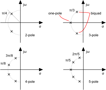
The problem of figuring out what the Q should be for each stage of a biquad cascade becomes very simple if we look at the pole positions of the Butterworth filter we want to achieve in the s-plane. In the s-plane, the poles of a Butterworth filter are distributed evenly, at a constant radius from the origin and with a constant angular spacing. Since the radius corresponds to frequency, and the pole angle corresponds to Q, we know that all of the component filters should be set to the same frequency, and their Q is simple to calculate from the pole angles. For a given pole angle, θ, Q is 1 / (2cos(θ)).
Calculating pole positions is easy: For a filter of order n, poles are spaced by an angle of π/n. For an odd order, we’ll have a one-pole filter on the real (horizontal) axis, and the remaining pole pairs spaced at the calculated angle. For even orders, the poles will be mirrored about the real axis, so the first pole pairs will start at plus and minus half the calculated angle. The biquad poles are conjugate pairs, corresponding to a single biquad, so we need only pay attention to the positive half for Q values.
Examples
For a 2-pole filter, a single biquad, the poles are π/2 radians apart, mirrored on both sides of the horizontal axis. So, our single Q value is based on the angle π/4; 1/(2cos(π/4)) equals a Q value of 0.7071.
For a 3-pole filter, the pole spacing angle is π/3 radians. We start with a one-pole filter on the real (σ) axis, so the biquad’s pole angle is π/3; 1/(2cos(π/3)) equals a Q of 1.0.
For a 4-pole filter, we have two biquads, with poles spaced π/4 radians apart, mirrored about the real axis. That means the first biquad’s pole angle is π/8, and the second is 3π/8, yielding Q values of 0.541196 and 1.306563.
Every time you post, I find that I learn something useful, or find that I have been thinking about something wrongly. That is the case here. Thank you Nigel!
Am I understanding this?
Let say you have a 2 pole LPF at 200Hz and a 2 pole HPF at 20Hz, basically your making a 20-200Hz bandpass 2 pole….
You calculate the co-efficients with Q=0.54119610 for the first filter and the output of that filter goes into 2nd filter with co-efficients with Q=1.3065630?
RichardS
No, this cascading is to make a single filter from multiple one- and two-pole filters. If you want to make a four-pole Butterworth lowpass with a corner of 200 Hz, you’d use two biquads set to a frequency of 200 Hz, and set the Q of each to the two values the calculator gives. Otherwise, the corner gets rounder and rounder as you cascade more biquads at the same frequency.
Coming back to your comment I am curious to know what is the best way to make a 4th order butterworth bandpass (e.g. 0.5-4.5 Hz). I suppose you can use your calculator with settings fc=1.5 and Q=0.375, but this will end up in 2nd order. How can you cascade a bandpass to come up with a 4th order? Reapply or alter somehow the Q factor?
Otherwise is it equal to use two-cascaded low-pass at 4.5Hz and two cascaded high-pass at 0.5 Hz?
Thanks a lot in advance for your time and the excellent calculator you provide.
Bandpass depends on who it is defined, so I don’t have a quick answer for that. But yes, you can cascade lowpass and highpass. However, note that you only need one 2nd order lowpass and one 2nd order highpass to give you a 4th order bandpass equivalent.
Assuming in the bandpass case Q is replaced by Bandwidth(octaves) and is user adjustable usually. Cascading LP/HP butterworths will not result in a butterworth bandpass, especially noticeable as bandwidth decreases ( I actually just tested this). Think Q/BW needs to be adjusted as the two bandedges/poles move closer. All solutions I’ve seen solve this in the analog domain/s-plane (Like Vinnie Falco’s filter library) before the BLT which breaks the simplicity of doing butterworths directly in digital. Is there an easier way?
I am on the same quest to find how are the Qs would be for bandpass and bandstop cases, and finally I have found it. In “Digital Audio Signal Processing” by Udo Zölzer, page 121, he clearly listed what the Q (pole quality factor) are for different filters. For Bandpass/stop, Q = fc/fb. So for a bandpass 0.5 Hz – 4.5 Hz, fc = 2.5 Hz, fb = 4 Hz, Q = 2.5/4…
The comment above contains error, fc is not the middle of bandwidth but rather the geometric mean of bandwidth, whereby fc = sqrt( f1 * f2 )
I have finally found out how to calculate the Q for cascaded Bandpass or Notch:
Q (each-stage) = Qintended * sqrt( 2 ^ ( 1 / number_of_biquad ) – 1 ), where,
Qintended = fc / bandwidth, and
fc = sqrt( f1 * f2 ) and bandwidth = ( f2 – f1 )
To supplement my previous comment and to do corrections:
fc is centre frequency which should be the centre of BW.
Qintended is rather = f0 / BW, where f0 is the “Geometric Mean”: f0 = sqrt(f1*f2)
The formula of how to calculate Q for each cascaded Biquad is obtained from Linear Technology Application Note an27af, 1988, ” A Simple Method of Designing Multiple Order All Pole Bandpass Filters by Cascading 2nd Order Sections”
And the way I calculated the coefficients is rather based on “Cookbook formulae for audio equalizer biquad filter coefficients” by Robert Bristow-Johnson, with alpha calculated based on Q (the EE-kind). I have not tried to Nigel’s method with the my set of Qs yet.
Cheers
This is a really useful formula, thanks for sharing the reference so I can check it. Now I’m testing it on my ESP32 platform and I’ll report it here. Have you tested the formula yourself and is it valid?
Just to let you know, I have tested it and it works. It doesn’t have flat response within the bandwidth but it’s fine for my application. Not recommended for wide bandwidth (more than 10% of the center frequency).
Would this work with simply cascading two of Andy Cytomics SVF filters to create a 4 pole lowpass? With the Q values given by your site?
Yes!
This is a really great blog, thank you for all the information. I wonder if this works with other filters than low-/highpass e.g. RBJ shelving or peaking filters.
This really only makes sense for lowpass and highpass—filters that space their poles evenly at a constant radius in the s-plane. The definition of Butterworth, maximally flat, doesn’t work for a peaking filter, for instance. It makes sense for a higher-order shelf, but I’d have to think about what that means, since you have two corners…
Thanks for all your great posts! Most videos and articles about DSP are impractical and math-heavy, and just make me feel like an idiot. Your articles make me understand it and want to jump into my editor and actually implement stuff in my projects!
I have found this site very insightful. I have implemented your algorithms and get expected responses for the filters designed (2, 4 and 10 pole LPF, HPF using the cascaded biquad), except I am getting noise floor artifacts that peak at the corner frequency. For example, a 400 Hz LPF, 10 pole. I used your Q calculator for the filters and when I run the filter, each filter coefficient is the same as you get (LPF = exact to 16 significant digits, HPF to 11 significant digits). Normal noise floor of my 1kHz signal is ~ 160 dBm and this “peak” is -45 dBm at 400 Hz with a 10 dBm 1kHz signal. Any thoughts where this may be coming in? All math is being done in doubles.
Also, I do remove the first 4 samples of my sample array after applying all cascaded filters, since the filter needs this many to initialize z1 and z2 correctly. I also put an impulse response into the filter and removed more points for settling, but the artifact still shows up (although a bit lower in response, say -76 dBm). I did see some change in behavior when changing the cascaded algorithm from not zeroing z1 and z2, to when I do. You don’t really mention anything about these parameters when cascading.
Is there a way to calculate the greatest steepness or effective order, given a certain precision? Let’s I am working with single precision floats, then possibly a 40th order is my effective limit while 60th order given double precision. Essentially, I would like to determine the maximum effective order. How close can you get to the brick wall?
Good question. Easier to just try it out though.
How do you calculate the angles for other Q values?
For example with Q=1 as apposed to .707, the angle will be 60°. How do you calculate the start angle for the poles here?
For Butterworth, the definition is clear (maximally flat passband), for arbitrary Q, I don’t know offhand, don’t want to guess, don’t have time to do some calculations to check. Obviously, the poles rotate towards the jw axis in the s-plane (and towards the unit circle in the z-plane), as you note, but I don’t know the motion of the other poles exactly.
Very nice article, it gives me deeper understanding!
Hope this will help people to find their biquads:
In MATLAB or octave(FREE), you can convert a “direct form” (higher order) quite easily to biquad using tf2sos()
tf2sos
Convert digital filter transfer function data to second-order sections form
For example
design your filter e.g.
pkg load signal
fs =48000
fn=fs/2
order=4
[cze,cpo]=butter(order,12000/fn)
freqz(cze,cpo,4096,fs)
ze = roots(cze)
po = roots(cpo)
tf(cze,cpo,1/fs)
yields this filter:
cze = 0.093981 0.375923 0.563885 0.375923 0.093981
cpo = 1.0000e+00 -3.6776e-16 4.8603e-01 -5.1255e-17 1.7665e-02
0.09398 z^4 + 0.3759 z^3 + 0.5639 z^2 + 0.3759 z + 0.09398
y1: ———————————————————-
z^4 – 3.678e-16 z^3 + 0.486 z^2 – 5.126e-17 z + 0.01766
and here it comes…:
tf2sos(cze,cpo)
will generate your biquads:
9.3981e-02 1.8796e-01 9.3981e-02 1.0000e+00 -5.5511e-17 3.9566e-02
1.0000e+00 2.0000e+00 1.0000e+00 1.0000e+00 -2.7756e-16 4.4646e-01
How do you calculate the Q values for cascading Butterworth HP filters with each other?
I implemented something for cascading LP filters and I get the correct results but it does not work with HP filters so the Q values cannot be the same.
Lowpass and highpass are symmetric, the poles are spread in the same way (zeros on opposite sides), so the calculation is the same. You can see the symmetry in the coefficients if you choose an Fc in the center of the band (12000 for 48000 sample rate), in the biquad calculator, and switch between lowpass and highpass. There’s a single sign change. Change Q to see they still match. (You can choose symmetric frequencies too—6000 and 18000, etc.) Something else is wrong if it’s not working out for highpass.
When I cascade two 2nd order lp filters I calculate the same coefficients and adjust their Q values which yields the correct results (check by MATLAB). When I do the same for a 4th order
hp filter I tried the same and it does not work properly. The coefficients of the single biquad are correct (same values as in your calculator) and it generates the same Q values like the ones for the 4th order lp which works as intended.
i dont understand all the questions and answers above about butterworth´s Q here.
a butterworth topology doesnt have a Q at all, so you should also not be able to calculate it.
Good question. A Butterworth filter don’t have a Q control, but it does have a Q, it’s 0.7071 (one over the square root of two). And if you take a fourth-order Buttterworth and factor it into two cascaded second order filters, you can’t use a Q of 0.7071 for each, that would be “Butterworth squared” (convenient for Linkwitz-Riley filters, though).
Hi Nigel,
thanks so much for this information. I’m trying to re-write history and getting confused. In 2009 we needed to match BW8 LPF and HPF sections with 4 cascaded Biquads – we used LEAP to simulate the responses and output coefficients. We then had to somehow transform them to enter into the DSP. Of course LEAP is no more so now, in trying to re-create the filter on another DSP platform, I can’t remember the process to reverse the transform. I wonder whether with your experience you might be able to take one look and tell me, based on the numbers below….which come straight out of the old DSP.
HPF Filter 1 Filter 2 Filter 3 Filter 4
bo 0.943228 0.872966 0.825878 0.802455
b1 -1.886455 -1.745931 -1.651758 -1.604910
b2 0.943228 0.872966 0.825878 0.802455
a0 1.860028 1.721473 1.628619 1.582428
a1 -0.912882 -0.770389 -0.674897 -0.627393
LPF Filter 1 Filter 2 Filter 3 Filter 4
bo 0.013212 0.012229 0.011568 0.011241
b1 0.026425 0.024458 0.023139 0.022483
b2 0.013212 0.012229 0.011568 0.011241
a0 1.860027 1.721473 1.628619 1.582428
a1 -0.912882 -0.770389 -0.674897 -0.627393
Hope you can help,
Best regards,
David
You can find the biquad equations elsewhere on the site (for instance, Biquad formulas). You’ll need to do some (ha) algebraic manipulation, of course, to solve in terms of Fc and Q. On the bright side, of the five coefficient equations, you only need three (for instance, the lowpass a1 and a2 are in terms of the others, and can be ignored). Next, you need to know your coefficient mapping, because it’s not standard. For that, the easiest thing to do is try an example with the Biquad calculator and jockey values until the coefficients match up. At the default 44.1 kHz rate, Fc = 1652 Hz and Q = 2.7 matches up roughly with the first lowpass coefficients, so we know the mapping of yours to mine is b0 -> a0, and therefore we can ignore b1 and b2, and a0 -> -b1 and b2 -> -a1. It might be easier to measure the filter response for the -3 dB point if you can. (Are you sure they are Butterworth, though? This looks suspiciously like a crossover problem, which is likely Butterworth-squared, two fourth-order Butterworth.)
Thanks Nigel – I’ll give it a crack!
Done – thanks so much for your help.
The 4 filters are 4 x variable Q filters (with Qs you describe on this page) which add to build a replica of a BW8 at 1800Hz at 48000Hz Fs pretty darn accurately.
I think I can proceed with confidence now. Hurrah.
David
Great!
This is awesome! This post saved my amateur ass the troubles of figuring out how to construct higer order filter from biquad sections properly.
Thank you!
This is immensely helpful, one of the very few resources I’ve been able to find that explicitly spells this out at all. I’m wondering does this same method extend to band pass and notch/band stop filters as well? After quick testing it doesn’t seem to be as simple as just using these Q values, but I assume there’s an analogous way to calculate similar series of values for these filter types as well to cascade higher order versions of them. Looking at the pole-zero plots however I couldn’t figure out any sort of a geometric interpretation of how the Q values should be calculated for appropriate cascading.
I don’t have an immediate answer for that. It’s a little different issue, since the article covers how to get a Butterworth response for higher orders of lowpass filters, made from first and second order sections. There is less call for high order Butterworth bandpass, I suppose.
From here is missing the equation. Q is variable parameter not fixed on 0.7, how to transform 2 poles biquad filter in 4 poles biquad filter ? From one Q variable parameter must have an equantion to calculate 2 parameters of Q for each filter in cascade.
Unlike the definition of a Butterworth filter, exactly how Q behaves in a filter is not precisely defined. For instance, the Moog lowpass filter is four one-pole filters with an overall feedback loop—you can’t do the same thing with two or three poles, for instance, and he Q of a biquad behaves differently. You could experiment with setting two biquads in series with the same parameters, for instance, and see if it gives you the response you want. If you’re looking for a four-pole synth filter, you’d be better off to look for a Moog-style implementation, or other four-pole filter. The value of cascading technique I’m showing here is not so much for four-pole filters, but for even higher order, where a single filter can run into numerical problems and it makes sense to split it over multiple lower-order (biquad and first order) filters.
If I want a peak filter with 24db/octave rather than 12db/oct where would I positino the poles? Is it a matter of constructing a 12db one first and then subdividing? I wonder if you had a rough idea on how to tackle this?
Thanks for this great resource!
Dave.
Se my reply to John Jenwty. The answer can be whatever you want it to be for a peaking filter, including simply to biquad peaking filters in series with the same settings (except you’d need to adjust for the combined gain). However, for a peaking filter, the steepness is generally controlled by Q, and higher order filters might not make sense musically.
Hi Nigel,
I found a single formula that applies to both even and odd orders:
https://github.com/antoineportes/DSP/blob/main/filters/Damping%20factors%20in%20Butterworth%20cascades
Interesting. With my method, the is only a single formula. I calculate the Q for the pole angle then use my standard formula to calculate each set of coefficients.