We look at what Pulse Amplitude Modulation added to our analog source audio.
What did PAM add?
Earlier, we noted that the PAM signal represents the the source signal plus some additional high frequency content that we need to remove with a lowpass filter before we listen back.
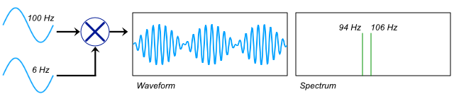
Again, PAM is amplitude modulation of the source signal with a pulse train. Mathematically, we know precisely what amplitude modulation produces—the sums and differences of every frequency component between the two input signals. That is, if you you multiply a 100 Hz sine wave by a 6 Hz sine wave, the result is the sum of 106 Hz and 94 Hz sine waves. For signals with more frequency components, there are more sums and differences in the result.
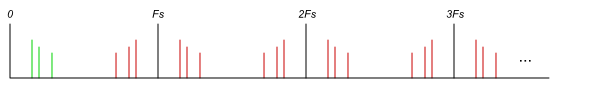
 To answer our question, “What got added?”, we need to understand the frequency content of a pulse train. One way to know that would be to use an Fourier Transform on the pulse train. But I want to use intuitive reasoning to eliminate as much math as possible. Fortunately, I already know what the extra frequency content is—it’s the spectral images in sampled systems, as described in classic DSP textbooks. That coupled with knowledge of amplitude modulation tips me off that we’ll need a frequency component at 0 Hz (DC—we need that to keep our original source band), at the sample rate, and at every integer multiple of the sample rate. Through infinity.
OK, we’ll lighten up on the infinity requirement. We can’t produce a perfect impulse in the analog world anyway. And we don’t need to. However, once in the digital domain, samples represent perfect impulses. While their values may have deviated slightly from a perfect representation of the analog signal, due to sampling time jitter and quantization, any math we do to them is “perfect” (again, subject to quantization and any other approximations). In the digital realm, the images do go to infinity.
Indeed, as you add cosine waves of 0, 1, 2, 3, 4…times the sample rate, the result gets closer and closer to the shape of an impulse. (Cosine instead of sine so that the peaks of the different frequencies line up.)
And that means we’ll have a copy of the source signal mirrored around 0 Hz, around the sample rate, twice the sample rate, three times the sample rate…to infinity. (In both directions, but we can ignore negative frequencies—for real signals, the negative spectrum mirrors the positive.)
What we’ve learned
Revisiting my “secrets”, with added comments:
1. Individual digital samples are impulses. Not bandlimited impulses, ideal ones.
Bothered that ideal impulses are impossible? Only in the physical world. There, we accept limitations. For instance, gather together infinity of something. Anything—I’ll wait. Meanwhile, in the mathematical world, infinity fits easily on this page: ∞
2. We know what lies between samples—virtual zero samples.
Think there’s really a continuous wave, implied, between samples? If so, you probably think it’s because samples represent a bandlimited impulse. No—you’re getting confused with what will come out of the DAC’s lowpass filter later, when we play back audio.
3. Audio samples don’t represent the source audio. They represent a modulated version of the audio. We modulated the audio to ensure points #1 and #2.
This is a frequency-domain observation that follows from the first two points, which are time domain. If you understand this point, you’ll never be confused about sample rate conversion.
Man great stuff very granular and tangible will be bookmarking this blog
could you please help me a little bit. I couldn’t grasp what you were telling here–“To answer our question, “What got added?”, we need to understand the frequency content of a pulse train. One way to know that would be to use an Fourier Transform on the pulse train. But I want to use intuitive reasoning to eliminate as much math as possible. Fortunately, I already know what the extra frequency content is—it’s the spectral images in sampled systems, as described in classic DSP textbooks. That coupled with knowledge of amplitude modulation tips me off that we’ll need a frequency component at 0 Hz (DC—we need that to keep our original source band), at the sample rate, and at every integer multiple of the sample rate. Through infinity.”
What gets added? You could point me towards some reference material if you have.
It’s the spectral images (the aliases of the original signal). What I’m getting at here is that the samples do not represent the original signal that was sampled, but a modulated version of it. How profound that is to you depends on how you intend to process the sampled audio. If it’s a linear filter, it’s not an issue (as long as filter gain doesn’t also clip the D/A converter on playback). But if you want to do sample rate conversion or non-linear processes, it’s important to understand “what got added”. I hope that’s a little clearer.
Nigel
Nigel, as an embedded sw engineer I decided a few years ago to move from the more boring MCU land to the exciting DSP land. For some reason, on the DSP side of the spectrum you meet lots of clever people, most of them are a bit ‘off’ for some reason. As it appears, you need some special gen for DSP engineering.
I believe only very few people have deep understanding of the math and physics in the signal processing world, while at the same time being able to explain those to mere mortals. You appear to be one such person and I’m in awe of that fact.
I appreciate that very much, Bart. I expect to have more a little more time in 2019, hope to more more active here soon, and especially tackle the long-awaited video…