Sampling theory, the best explanation you’ve ever heard—Part 1

I’ll start by giving away secrets first:

  1. Individual digital samples are impulses. Not bandlimited impulses, ideal ones.
  2. We know what lies between samples—virtual zero samples.
  3. Audio samples don’t represent the source audio. They represent a modulated version of the audio. We modulated the audio to ensure points #1 and #2.

Well, not secrets, but many smart people—people who’ve done DSP programming for years—don’t know these points. They have other beliefs that have served them well, but have left gaps.

Let’s see why

Analog audio, to digital for processing and storage, and back to analog

Component details—first the analog-to-digital converter (ADC)

The digital-to-analog converter (DAC)

Analog to digital conversion, and conversion back to analog are symmetrical processes—not surprising.

But we can make another important observation: We know that the bandlimiting lowpass filter of the ADC is there as a precaution, to ensure that the source signal is limited to frequencies below half the sample rate. But we have an identical filter at the output of the DAC—why do we need that, after eliminating the higher frequencies at the beginning of the ADC? The answer is that conversion to discrete time adds high frequency components not in the original signal.

Stop and think about this—it’s key to understanding digital audio. It means that the digital audio samples do not represent the spectrum of the bandlimited analog signal—the samples represent the spectrum of the bandlimited analog signal and additional higher frequencies.

To understand the nature of the higher frequencies added in the sampling process, it helps to look at the origins of sampling.

Next: We explore the origins of sampling in Part 2

Posted in Digital Audio, Sampling Theory | Tagged | 4 Comments

Sampling theory, the best explanation you’ve ever heard—Prologue

I’ve been working on a new video, with the goal of giving the best explanation of digital sampling you’ve ever heard. The catch is I started on it three years ago. I’m not that slow, it’s just that I’ve been busy with projects, so time passes between working on it. And each time I get back to it, I rewrite it from scratch. You see, I want to give you a solid, useful theoretical framework that will both help you understand and help you make good decisions, with the goal of being intuitive. So, each time I have a little different viewpoint to try.

The video is still a few months off—I’m still busy for the next few months—but I’m going to present the idea first as a collection of short articles. And in the end, if I like it, the articles will serve as the script for the video.

I believe this is a unique explanation of sampling. Please follow it from the start, even if you feel you know the subject well. This isn’t something I read or was taught, but came from thinking about a way to explain it without descending into either mathematical symbolism or hand waving.

Next up: My first crack at the best explanation of sampling theory you’ve ever heard.

Posted in Digital Audio, Sampling Theory | Tagged | Leave a comment

Amp simulation oversampling

In tandem with our last article on Guitar amp simulation, this article gives a step by step view of the sampling and rate conversion processes, with a look at the frequency spectrum.

From guitar to digital

The first two charts embody the initial sampling of the analog signal. It’s done in one step, from your analog-to-digital converter, but it’s a two-part process. First, a lowpass filter clears everything from half the sample rate up—something we must do to avoid higher frequencies aliasing into our audio band when sampled.

Then the signal is digitized. This creates repeating images of the positive and negative frequencies that extend upward without end. After this, we’ll look only at frequencies between 0 Hz and the sampling frequency, but it’s important to understand that these images are there, nonetheless.

If we don’t need more frequency headroom, we can do our signal processing on the samples we have. In fact, we want to do as much as we can at the lower sample rate. In the case of a guitar amp, we would process any tone controls that come before the “tube”, and other things like DC blocking and noise gating. And we can do our (non-saturating) gain stage here (assuming floating point).

Higher rate processing

After initial processing and gain, it’s time for saturation. For this non-linear process, we need frequency headroom. The first step is to increase the rate by inserting zero-magnitude samples. Though I suggested starting with 8x upsampling in the guitar amp article, this exercise shows 4x, in order to better accommodate page constraints. We place three zero-samples between each existing sample to bring it up 4x. This only raises the sample rate—we have four samples in the same period that we used to have one. Since the spectrum is not altered, the aliases are still there.

Part two of the sample rate conversion process is to use a lowpass filter to clear everything above our original audio band. (In reality, we optimize the zero insertion and filtering into a single process, to take advantage of multiplies by zero that we can skip. Note we usually use a linear-phase FIR for this step, in order to preserve the wave shape for the saturator.) Now we see our headroom.

After our saturation stage, we’ve created new harmonics. As long as they are at a sufficiently low level by the time they reach the sample rate minus our final audio bandwidth, the aliased version won’t pollute our audio band.

Back to normal

Done with our more expensive high-rate signal processing, we can drop back to our original sample rate for the rest. The first step is to run our lowpass filter again, to clear everything above our audio band.

Part two is the downsampling process—we simply keep one sample, discard three, and repeat. Why did we bother calculating them? Because we needed them ahead of the lowpass filter. But, here also, we can optimize these two down-conversion steps into one, and save needless calculation.

Final processing

From here, we handle other linear processes—any filtering and tone controls the follow the tube stage, effects such spring reverb, and finally the speaker cabinet simulation. In the end, we send it to our digital-to-analog converter, which itself has a lowpass filter to remove the aliased copies.

And enjoy listening.

Posted in Digital Audio, Effects, Guitar Amp Simulation, Sample Rate Conversion | 4 Comments

Guitar amp simulation

In this article, I’ll sketch a basic guitar amp simulator. For one, questions on the topic come up often, and also, it will be a good example of a typical use of working at a higher sample rate.

The most basic guitar amp simulator has gain, with saturation, tone controls, and a speaker cabinet simulator. Because saturation is a non-linear process, the results are different whether the tone controls come before or after—more on this later. The speaker cabinet, of course, comes last, and is an important part of the tone. Gain with saturation (the overdriven “tube”) is the tricky part—we’ll start there.

Gain with saturation

Gain is simply a multiply. But we like to overdrive guitar amps. That means gain and some form of clipping or softer limiting—that’s what generates the overdrive distortion harmonics we want. Typically, we’d ease into the clipping, more like tube saturation behaves, but the more overdrive gain you use, the closer it gets to hard clipping, as more of the signal is at the hard limit.

That’s where we hit our first DSP problem. Clipping creates harmonics, and there’s no way to say, “Please, only generate harmonics below half the sample rate.” We will have aliasing. The added harmonics fall off in intensity (in much the same way as harmonics of a rectangular wave do), as they extend higher in frequency, but at typical digital audio sample rates, the Nyquist Frequency comes too soon. Aliased images extend back down into the audio range. We can’t filter them out, because they mix with harmonics we want to keep. And because the guitar notes played aren’t likely the be an integer multiple of the sample period, the aliased harmonics are out of tune. Worse, if you bend a guitar note up, the aliased harmonics bend down—that’s where aliasing becomes painfully apparent.

Can we calculate clipping overtones and create just the ones we want? Can we analyze the input and output and remove frequencies that we don’t want? That is not an easy task (left as an exercise for the reader!).

The oversampled solution

To mitigate the aliasing issue, the most practical solution is to give ourselves more frequency headroom before generating distortion harmonics with our saturation stage. If the sample rate is high enough, aliased images are spread far enough apart that the tones extending into our audio range from above are diminished to the point they are obscured by the din of our magnificent, thick, overdriven guitar sound. And when we play delicately or with little overdrive gain, so is the aliasing lessened.

How much headroom?

How much headroom do we need? I’d like to leave that to your situation and experimentation—mostly. But since I started doing this in the days when every DSP cycle was a precious commodity, I can tell you that—for 44.1 kHz sample rate, typically the worst case that we care about—the minimum acceptable oversampling factor is 6x. 8x is a good place to start, and will be adequate for many uses, at a reasonable cost. (Do multistage oversampling for efficiency…but that’s another story.)

Raising the sample rate “8x” sounds like we’ll have eight times the bandwidth, but it’s better than that. At our original 44.1 kHz sample rate, we have a usable bandwidth of about 20 kHz (allowing for the conversion filters), and little addition frequency headroom. If we go past 24.1 kHz (44.1 kHz – 20 kHz), aliasing extends below 20 kHz. But by raising the rate to 8 times the original, we have headroom of 352.8 kHz – 20 kHz, or 332.8 kHz. That’s more than 80 times our original headroom.

The idea is that we upsample the signal (removing anything not in our original audio band), run it though our tube simulator (clipper/saturator), then drop the sample rate back to the original rate (part of this process is again removing frequencies higher than out original audio band).

How much gain?

Real guitar amps have a lot of gain. Don’t think that if your overdrive is adjustable from 0-2 gain factor, you’ll get some good overdrive distortion. That’s only a maximum of 6 dB. More like 60 dB (0-1024)! Maybe up to something like 90 dB for modern, screaming high-gain amps. That’s equivalent to a shift of 15 bits, so I hope you’re using something better than a 16-bit converter (or tracks) to input your raw guitar sound.

The tube

My intent here is not to guide you down the road of yet another guitar amp simulator plugin, but to give an example of a task that needed more frequency headroom, requiring processing at a higher sample rate. But it’s worth going into just a bit of detail on the tube (saturation) element. Again, we’re talking about “first approximations”—a hard clipper, or a soft one.

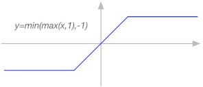
A hard clipper is trivial. If a sample is greater than 1, change it to 1. If less than -1, change it to -1.

if (samp > 1.0)
 samp = 1.0;
else if (samp < -1.0)
  sample = -1.0;

Here’s the transfer function—for input sample values along the x axis, the output is on the y axis. For input { 0.5, 0.8, 1.0, 1.3, 4.2 }, the output is { 0.5, 0.8, 1.0, 1.0, 1.0 }.

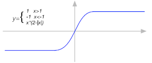
But for this use we’d probably like a softer clip—a transfer function that eases in to the limit. samp = samp > 1 ? 1 : (samp <= -1 ? -1 : samp * (2 – fabs(samp))); This is just a compact way of saying,

if (samp > 1.0)
  samp = 1.0;
else if (samp < -1.0)
  sample = -1.0;
else
  samp = samp * (2 - fabs(samp));

This is a very mild, symmetrical x-squared curve. It’s just an example, but you’ll find it produces useful results. You could try a curve that stays straighter, then curves quicker near +/-1. Or a curve that’s not symmetrical for positive and negative excursions. The harder the curve, the closer we get to our original hard-clipping.

One detail worth noting: If you’ve spent much time looking at discussions of this sort of non-linear transfer function on the web, usenet, or mailing lists, invariably someone points out that we know exactly what order of harmonics will be created, and therefore how much oversampling we might need, based on the polynomial degree. This is wrong—in fact we’re only using the polynomial between the bounds of x from -1 to 1, and substituting a hard clip for all other points. For a use such as this, the input is driven far into the hard clip region, so the polynomial degree is no longer relevant.

Tone controls

We know IIR filters well, so this part is easy. Typically, a guitar amp might have bass, mid, and treble controls. One catch is that if you want to sound like a particular vintage amp, they used passive filters that result in control interaction. That is, not active circuitry that isolate the components from each other. So, adjusting the bass band might affect the mid filtering as well. But that’s fairly easy to adjust for.

More about overdrive and tone

Something worth noting. It you really want to scream with gain, you need to make some architectural adjustments. If you’ve played much with raw distortion pedals with different instruments, you’ve probably noticed that you get a “flatulent” sound with heavy clipping of bass. And high-gain distortion of signals with a lot of highs can sound pretty shrill. Guitar solos really scream when they have a lot of midrange distortion. So, if you really want to go for a screaming lead with loads of distortion without it falling apart into useless grunge, one thing you can do is roll off the lows and highs before the tube sim (distortion) stage. But then the result lacks body—compensate by boost the lows and high back up, after the distortion stage. The point here is that you have three choices of where to put EQ for your amp tone: before the tube, after, or both.

Some of your tone choices can be a property of the amp model—not everything needs to be a knob for the user to control. These choices are what give a particular guitar amp its characteristics. A Fender Twin does not sound like a Marshall Plexi. The reason that well-known guitar amps are the basis of DSP-based simulation is that the choices of their designers have withstood the test of time. Countless competitors faded from memory, often because there choices were as compelling.

Cabinet

Similarly, guitar speakers gained familiar configurations not because the industry got together and chose, but these are the ones that worked out well.

One characteristic of speakers for guitar amps is that they are not full range—you’ll find no tweeters in guitar cabinets. The highs of the large speakers used (most often 10″ and 12″) drop off very quickly. A clean guitar tone doesn’t have strong high frequency harmonics, and the highest note on a guitar is typically below 1 kHz. Overdrive distortion creates powerful high frequency harmonics, but we really don’t want to hear them up very high—extremely harsh and fatiguing to listen to.

The first approximation of a speaker cabinet is simply a lowpass filter, set to maybe 5 kHz. I didn’t say it would be a great cabinet, but it would start to sound like a real guitar amp combo. The next step might be to approximate the response of a real speaker cabinet, miked, with multiple filters.

But if you’re serious, a better start might be to generate impulse responses of various cabinets (4 x 12″, 2 x 10″, etc.), miked at typical positions (center, edge, close, far), with selected mics (dynamic, condenser). Then use convolution to recreate the responses.

Followup

To moderate the size of this article, I’ll follow with images depicting the oversampling process in the next article.

Posted in Aliasing, Digital Audio, Sample Rate Conversion | 3 Comments

About coefficient conventions

It’s been asked many times, so it’s worth an article explaining the conventions used on this site for transfer functions, and why they may differ from what you see elsewhere.

People run into this most often with biquads: I use a (a0, a1, a2) in the numerator (defining zeros), and b in the denominator (defining poles). Many references, including wikipedia, use the opposite convention. Why am I so contrary?

OK, I go back a few years, back when the only way to find out about digital signal processing was to buy a college text book and try to make sense of it. In the beginning, there was no convention (I’m not sure there is now, other than de facto—please let me know if some technical society or other has put down the word). When I first went to write for the public, I took a survey of my book shelf. Most had a on top. And that choice made sense to me—a then b, from top to bottom, and also left to right for the direct form I structure. Finally, it makes sense that FIRs would have only a coefficients. Having only b coefficients seems odd, if you were to specialize the general transfer function.

My only guess for the other way preference, initially at least, is that when using the canonical (minimum number of delay elements) director form II, the result would be ab left to right.

So, I wrote a number of articles over the years using that convention. And over the years it seems that b-on-top has become dominant. (I recall seeing a-on-top on another major internet resource recently, and I see that one site even uses c and d—I assume to avoid the conflict altogether.) Free time is not something I have a lot of, so I don’t intend to edit all my articles, diagrams, and widgets to change the convention. I’m not saying it will never happen, but not for now.

It’s easy enough to notice which convention is used if you’re aware that there is no 100% agreement. Biquads (and higher order IIRs) are typically normalized to the output, making b0 (in my case) unity, so there is no coefficient needed. If you see a set of a and b coefficients, and a0 is missing and b0 is not, then the order is swapped relative to mine.

Finally, there is one other place that you can get caught with filter coefficients. When deriving a difference equation (y(n) = a0x(n) + a1x(n-1) + a2x(n-2) – b1y(n-1) – b2y(n-2)), sometimes people roll the minus signs for the feedback part into the respective coefficients. This damages the mathematical purity of it all a tad, but makes sense in a computer implementation. I don’t merge the minus signs—and fortunately, I don’t think most internet sources do either.

For the record, I’ll consult my bookshelf and see if I can come up with that original survey I mentioned earlier:

a on top

Theory and Application of Digital Signal Processing, Rabiner and Gold, 1975
Principles of Digital Audio—Second Edition, Pohlmann, 1989*
Advanced Digital Audio, Pohlmann, 1991
Digital Signal Processing—A Practical Approach, Ifeachor and Jervis, 1993
Digital Audio Signal Processing, Zölzer, 1997
Digital Signal Processing—An Anthology: Chapter 2, An Introduction to Digital Filter Theory, Julius O. Smith, 1983

* The topic doesn’t appear in the first edition. Also, although the text uses a for the top (forward path of the difference equations, actually), a diagram of the direct form II structure shows the opposite. Since Pohlmann is consistent, otherwise, it seems the diagram was taken from somewhere else.

b on top

I thought I had a few—can’t find any at the moment. Perhaps TI and Motorola application notes?

N on top, D on bottom (Numerator and Denominator!)

Multirate Digital Signal Processing, Rochiere and Rabiner, 1983

Other (these don’t use indexed coefficients)

Digital signal Analysis, Sterns, 1975
Musical Applications of Microprocessors, Chamberlin, 1980

Final notes

Again, the textbook survey is to show why I made the choice then, not to support why it should be that way now. Be aware that you can’t assume that a given author is consistent over time. Rabiner’s books use different conventions, with different co-authors, as noted. Julius O. Smith’s detailed 1983 article has a on top, while his vast web resources use b on top. In DAFX: Digital Audio Effects (like Anthology above, a collection from multiple authors), Zölzer has b on top. It’s always a good idea to pay attention—there is nothing magical about the coefficient naming, it’s simply a style consideration.

Posted in Biquads, IIR Filters | 7 Comments

Filter frequency response grapher

Here’s a tool that plots frequency response from filter coefficients.

Hz
Plot
Max
Range
a coefficients (zeros)
b coefficients (poles)

The coefficients fields are tolerant of input format. Most characters that don’t look like numbers are treated as separators. So, you can enter coefficients separated by spaces or commas, or on different lines, separated by returns. That makes it easier to copy and paste coefficients from online filter calculators. They also ignore numbers that are followed by “=” or “ =”, so that “a0 = 0.1234” is seen as “0.1234”. Click the chart to accept coefficient changes, or change one of the controls.

Important: This tool does not assume that the filter coefficients are normalized to y0. So, in most cases you’ll need to insert a “1” as the first pole coefficient, the b0 term.

If there are no pole coefficients, it’s an FIR filter—all zeros.

Again, the convention of this website is that coefficients corresponding to zeros (left side of a direct form I) are the a coefficients, and poles the b coefficients. It’s usually easy to see because most IIR filter calculators normalize the output. So, if you are missing a0, it probably means that a and b are swapped with respect to this site’s convention—just paste them in the opposite coefficients fields (and remember to use a 1 for the missing coefficient). Also, negative signs at the summation for the feedback terms (b) are not rolled into the coefficients.

Posted in Biquads, Filters, FIR Filters, IIR Filters, Widgets | 15 Comments

Evaluating filter frequency response

A question that pops up for many DSP-ers working with IIR and FIR filters, I think, is how to look at a filter’s frequency and phase response. For many, maybe they’ve calculated filter coefficients with something like the biquad calculator on this site, or maybe they’ve used a MATLAB, Octave, Python (with the scipy library) and functions like freqz to compute and plot responses. But what if you want to code your own, perhaps to plot within a plugin written in c++?

You can find methods of calculating biquads, for instance, but here we’ll discuss a general solution. Fortunately, the general solution is easier to understand than starting with an equation that may have been optimized for a specific task, such as plotting biquad response.

Plotting an impulse response

One way we could approach it is to plot the impulse response of the filter. That works for any linear, time-invariant process, and a fixed filter qualifies. One problem is that we don’t know how long the impulse response might be, for an arbitrary filter. IIR (Infinite Impulse Response) filters can have a very long impulse response, as the name implies. We can feed a 1.0 sample followed by 0.0 samples to obtain the impulse response of the filter. While we don’t know how long it will be, we could take a long impulse response, perhaps windowing it, use an FFT to convert it to the frequency domain, and get a pretty good picture. But it’s not perfect.

For an FIR (Finite Impulse Response) filter, though, the results are precise. And the impulse response is equal to the coefficients themselves. So:

For the FIR, we simply run the coefficients through an FFT, and take the absolute value of the complex result to get the magnitude response.

(The FFT requires a power-of-2 length, so we’d need to append zeros to fill, or use a DFT. But we probably want to append zeros anyway, to get more frequency points out for our graph.)

Plotting the filter precisely

Let’s look for a more precise way to plot an arbitrary filter’s response, which might be IIR. Fortunately, if we have the filter coefficients, we have everything we need, because we have the filter’s transfer function, from which we can calculate a response for any frequency.

The transfer function of an IIR filter is given by

\(H(z)=\frac{a_{0}z^{0}+a_{1}z^{-1}+a_{2}z^{-2}…}{b_{0}z^{0}+b_{1}z^{-1}+b_{2}z^{-2}…}\)

z0 is 1, of course, as is any value raised to the power of 0. And for normalized biquads, b0 is always 1, but I’ll leave it here for generality—you’ll see why soon.

To translate that to an analog response, we substitute e for z, where ω is 2π*freq, with freq being the normalized frequency, or frequency/samplerate:

\(H(e^{j\omega})=\frac{a_{0}e^{0j\omega}+a_{1}e^{-1j\omega}+a_{2}e^{-2j\omega}…}{b_{0}e^{0j\omega}+b_{1}e^{-1j\omega}+b_{2}e^{-2j\omega}…}\)

Again, e0jω is simply 1.0, but left so you can see the pattern. Here it is restated using summations of an arbitrary number of poles and zeros:

\(H(e^{j\omega})=\frac{\sum_{n=0}^{N}a_{n}e^{-nj\omega}}{\sum_{m=0}^{M}b_{m}e^{-mj\omega}}\)

For any angular frequency, ω, we can solve H(e). A normalized frequency of 0.5 is half the sample rate, so we probably want to step it from 0 to 0.5—ω from 0 to π—for however many points we want to evaluate and plot.

Coding it

From that last equation, we can see that a single FOR loop will handle the top or the bottom coefficient sets. Here, we’ll code that into a function that can evaluate either zeros (a terms) or poles (b terms). We’ll refer to this as our direct evaluation function, since it evaluates the coefficients directly (as opposed to evaluating an impulse response).

You’ve probably noticed the j, meaning an imaginary part of a complex number—the output will be complex. That’s OK, the output of an FFT is complex too, and we know how to get magnitude and phase from it already.

Some languages support complex arithmetic, and have no problem evaluating “e**(-2*j*0.5)”—either directly, or with an “exp” (exponential) function. It’s pretty easy in Python, for instance. (Something like, coef[idx] * math.e**(-idx * w * 1j), as the variable idx steps through the coefficients array.)

For languages that don’t, we can use Euler’s formula, ejx = cos(x) + j * sin(x); that is, the real part is the cosine of the argument, and the imaginary part is the sine of it.

(Remember, j is the same as i—electrical engineers already used i to symbolize current, so they diverged from physicists and used j. Computer programming often use j, maybe because i is a commonly used index variable.)

So, we create our function, run it on the numerator coefficients for a given frequency, run it again on the denominator coefficients, and divide the two. The result will be complex—taking the absolute value gives us the magnitude response at that frequency.

Revisiting the FIR

Since we already had a precise method of looking at FIR response via the FFT/DFT, let’s compare the two methods to see how similar they are.

To use our new method for the case of an FIR, we note that the denominator is simply 1, so there is no denominator to evaluate, no need for division. So:

For the FIR, we simply run the coefficients through our evaluation function, and take the absolute value of the complex result to get the magnitude response.

Does that sound familiar? It’s the same process we outlined using the FFT.

And back to IIR

OK, we just showed that our new evaluation function and the FFT are equivalent. (There is a difference—our evaluation function can check the response at an arbitrary frequency, whereas the FFT frequency spacing is defined by the FFT size, but we’ll set that aside for the moment. For a given frequency, the two produce identical results.)

Now, if the direct evaluation function and the FFT give the same results, for the same frequency point, and the numerator and denominator are evaluated by the same function, by extension we could also get a precise evaluation by substituting an FFT process for both the numerator and denominator, and dividing the two as before. Note that we’re no longer talking about the FFT of the impulse response, but the coefficients themselves. That means we no longer have the problem of getting the response of an impulse that can ring out for an unknown time—we have a known number of coefficients to run through the FFT.

Which is better?

In general, the answer is our direct evaluation method. Why? We can decide exactly where we want to evaluate each point. That means that we can just as easily plot with log frequency as we can linear.

But, there may be times that the FFT is more suitable—it is extremely efficient for power-of-2 lengths. (And don’t forget that we can use a real FFT—the upper half of the general FFT results would mirror the lower half and not be needed.)

An implementation

We probably want to evaluate ω from 0 to π, corresponding to a range of half the sample rate. So, we’d call the evaluation function with the numerator coefficients and with the denominator coefficients, for every ω that we want to know (spacing can be linear or log), and divide the two. For frequency response, we’d take the absolute value (equivalently, the square root of the sum of the squared real and imaginary parts) of each complex result to obtain magnitude, and arc tangent of the imaginary part divided by the real part (specifically, we use the atan2 function, which takes into account quadrants). Note that this is the same conversion we use for FFT results, as you can see in my article, A gentle introduction to the FFT.

\(magnitude:=\left |H \right |=abs(H)=\sqrt{H.real^2+H.imag^2}\)
\(phase := atan2(H.imag,H.real)\)

For now, I’ll leave you with some Python code, as it’s cleaner and leaner than a C or C++ implementation. It will make it easier to transfer to any language you might want (Python can be quite compact and elegant—I’m going for easy to understand and translate with this code). Here’s the direct evaluation routine corresponding to the summation part of the equation (you’ll also need to “import numpy” to have e available—also available in the math library, but we’ll use numpy later, so we’ll stick with numpy alone):

import numpy as np

# direct evaluation of coefficients at a given angular frequency
def coefsEval(coefs, w):
    res = 0
    idx = 0
    for x in coefs:
        res += x * np.e**(-idx * 1j * w)
        idx += 1
    return res

Again, we call this with the coefficients for each frequency of interest. Once for the numerator coefficients (the a coefficients on this website, corresponding to zeros), once for the denominator coefficients (b, for the poles—and don’t forget that if there is no b0, the case for a normalized filter, insert a 1.0 in its place). Divide the first result by the second. Use use abs (or equivalent) for magnitude and atan2 for phase on the result. Repeat for every frequency of interest.

Here’s a python function that evaluates numerator and denominator coefficients at an arbitrary number of points from 0 to π radians, with equal spacing, returning arrays of magnitude (in dB) and phase (in radian, between +/- π):

# filter response, evaluated at numPoints from 0-pi, inclusive
def filterEval(zeros, poles, numPoints):
    magdB = np.empty(0)
    phase = np.empty(0)
    for jdx in range(0, numPoints):
        w = jdx * math.pi / (numPoints - 1)
        resZeros = coefsEval(zeros, w)
        resPoles = coefsEval(poles, w)

        # output magnitude in dB, phase in radians
        Hw = resZeros / resPoles
        mag = abs(Hw)
        if mag == 0:
            mag = 0.0000000001  # limit to -200 dB for log
        magdB = np.append(magdB, 20 * np.log10(mag))
        phase = np.append(phase, math.atan2(Hw.imag, Hw.real))
    return (magdB, phase)

Here’s an example of evaluating biquad coefficients at 64 evenly spaced frequencies from 0 Hz to half the sample rate (these coefficients are right out of the biquad calculator on this website—don’t forget to include b0 = 1.0):

zeros = [ 0.2513643668578741, 0.5027287337157482, 0.2513643668578741 ]
poles = [ 1.0, -0.17123074520885395, 0.1766882126403502 ]

(magdB, phase) = filterEval(zeros, poles, 64)

print("\nMagnitude:\n")
for x in magdB:
    print(x)

print("\nPhase:\n")
for x in phase:
    print(x)

Next up, a javascript widget to plot magnitude and phase of arbitrary filter coefficients.

Extra credit

The direct evaluation function performs a Fourier analysis at a frequency of interest. For better understanding, reconcile it with the discrete Fourier transform described in A gentle introduction to the FFT. In that article, I describe probing the signal with cosine and sine waves to obtain the response at a given frequency. Look again at Euler’s formula, which shows that e is cosine (real part) and sine (imaginary part), which the article alludes to this under the section “Getting complex”. You should understand that the direct evaluation function presented here could be used to produce a DFT (given complete evaluation of the signals at appropriately spaced frequencies). The main difference is that for this analysis, we need not do a complete and reversible transform—we need only analyze frequency response values that we want to graph.

Posted in Biquads, FFT, Filters, FIR Filters, IIR Filters | 27 Comments

Cascading filters

Sometimes we’d like to cascade biquads to get a higher filter order. This calculator gives the Q values for each filter to achieve Butterworth response for lowpass and highpass filters.

Order:
Q values:

You can calculate coefficients for all biquad (and one-pole) filters with the biquad calculator.

Motivation for cascading filters

Sometimes we’d like a steeper cutoff than a biquad—a second order filter—gives us. We could design a higher order filter directly, but the direct forms suffer from numerical problems due to limited computational precision. So, we typically combine one- and two-pole (biquad) filters to get the order we need. The lower order filters are less sensitive to precision errors. And we maintain the same number of math operations and delay elements as the equivalent higher order filter, so think of cascading as simply rearranging the math.

Adjusting the corner

The main problem with cascading is that if you take two Buterworth filters in cascade, the result is no longer Butterworth. Consider a Butterworth—maximally flat passband—lowpass filter. At the defined corner frequency, the magnitude response is -3 dB. If you cascade two of these filter, the response is now -6 dB. We can’t simply move the frequency up to compensate, since the slope into the corner is also not as sharp. Increasing the Q of both filters to sharpen the corner would degrade the passband’s flatness. We need a combination of Q values to get the correct Butterworth response.

How to calculate Q values

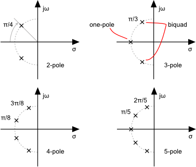
The problem of figuring out what the Q should be for each stage of a biquad cascade becomes very simple if we look at the pole positions of the Butterworth filter we want to achieve in the s-plane. In the s-plane, the poles of a Butterworth filter are distributed evenly, at a constant radius from the origin and with a constant angular spacing. Since the radius corresponds to frequency, and the pole angle corresponds to Q, we know that all of the component filters should be set to the same frequency, and their Q is simple to calculate from the pole angles. For a given pole angle, θ, Q is 1 / (2cos(θ)).

Calculating pole positions is easy: For a filter of order n, poles are spaced by an angle of π/n. For an odd order, we’ll have a one-pole filter on the real (horizontal) axis, and the remaining pole pairs spaced at the calculated angle. For even orders, the poles will be mirrored about the real axis, so the first pole pairs will start at plus and minus half the calculated angle. The biquad poles are conjugate pairs, corresponding to a single biquad, so we need only pay attention to the positive half for Q values.

Examples

For a 2-pole filter, a single biquad, the poles are π/2 radians apart, mirrored on both sides of the horizontal axis. So, our single Q value is based on the angle π/4; 1/(2cos(π/4)) equals a Q value of 0.7071.

For a 3-pole filter, the pole spacing angle is π/3 radians. We start with a one-pole filter on the real (σ) axis, so the biquad’s pole angle is π/3; 1/(2cos(π/3)) equals a Q of 1.0.

For a 4-pole filter, we have two biquads, with poles spaced π/4 radians apart, mirrored about the real axis. That means the first biquad’s pole angle is π/8, and the second is 3π/8, yielding Q values of 0.541196 and 1.306563.

s-plane-filters

Posted in Biquads, Filters, IIR Filters, Widgets | 40 Comments

Filters for synths—the 4-pole

The last post noted that the two most popular synthesizer filters are the 2-pole state variable, and the 4-pole “Moog style”. And we started with the state variable—simple, popular, and delivering multiple filter outputs (lowpass, bandpass…) simultaneously. Here, we’ll follow up with comments on the filter associated with Moog (and especially the Minimoog). In general, we’ll refer to this as a 4-pole synth filter.

While this filter is usually thought of as a lowpass filter, the other popular filter types can be derived easily. Many people first saw this in the Oberheim Xpander (and Matrix-12) synths of the ’80s, the idea came from Bernie Hutchins’ Electronotes in the ’70s. So don’t feel that you must go the direction of the state variable is you want multiple filter types, including 2-pole response.

Lowpass response is the overwhelming choice for typical synth use. Note that a 4-pole lowpass is not necessarily better then a 2-pole (as in the state variable)—they are just choices. You might want a 4-pole for the darker Minimoog bass sounds, and a 2-pole for the brassy OB8-style sounds.

Basic construction

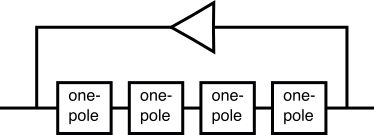
The 4-pole is implemented by a string of four one-pole lowpass filter in series. We need corner peaking and resonance control for a synth filter, and we get that by feeding back the output to the input. While trivial in the analog domain, this feedback is the tricky part in the digital recreations. The reason is that it’s not a continuous system, and the obvious way to handle it is to put a delay in that part, so the output of the current sample period is available as input for the next. But this creates some bad side effects, particularly for tuning. In the past, people dealt with this by accounting for those errors.
4-pole

Approaching analog

But it’s not just tuning errors—if it were, that would be simple to fix. The Minimoog popularity, in part, is that it is designed to easily overdrive the filter, to get a “fat” tone. This is another thing that is simple in the analog domain, but doing the same in the digital domain produces noticeably digital artifacts. And if your goal is to make something that sound analog, this is a source of spectacular “fail”.

So instead of this simple delay approach in the 4-pole feedback path, modern ideas use more complex techniques to avoid the large-scale errors in an effort to get closer to how the analog counterpart works. And part of the effort is in dealing with an overdriven feedback path. The result reduced digital artifacts, makes the filter’s behavior more closely resemble its analog counterpart when overdriven, and also gives a smoother, more predictable and more musical sound at high resonance.

Note that these techniques are often called “zero feedback delay” (ZDF) filters. That is meant to highlight the fact a trivial delay is not used. I’m not a huge fan of that, since it’s not meaningful to someone who doesn’t know of the delay it refers to, and of course there are always sources of internal delay in an such filter design. But I mention ZDF so that if you’ve heard it before, be assured that we are talking about those sort of techniques here.

Serious reading

A great resource for this topic is Vadim Zavalishin’s The Art of VA Filter Design (“VA” for “Virtual Analog”).

Posted in Digital Audio, Filters, IIR Filters, Synthesizers | 5 Comments

Filters for synths–starting out

We haven’t developed a synth filter here yet…

Filters we’ve presented

Biquads. While they are useful for many simple cases of filtering, they are not a good choice for analog synthesizer emulation. Most notably, they are poorly suited to time-varying parameters such as smooth filter sweeps.

Hal Chamberlin’s digital state variable filter, which has the advantage of independent control of filter frequency and resonance (Q), as well as simultaneous output of lowpass, bandpass, highpass, and notch filtering. While this served in many synthesizers over the years, using oversampling to fix its most glaring problem (limited frequency control range before losing stability), more modern design approaches offer far better performance.

What analog synths use

It’s helpful to discuss what most people are used to before getting to digital implementations.

For analog synthesizer emulation, two basic analog designs stand out, having withstood the test of time the best. The 24 dB/octave (“four pole”) Moog style (“transistor ladder”) lowpass filter, and the 12 dB/octave (“two pole”) state variable with its multiple outputs.

There are other designs, including the “diode ladder” design by Roland, the Steiner-Parker filter (basically Sallen-Key)—these are some of the ways voltage control was solved in analog filters, resulting in characteristic sounds. We’ll limit discussion to the two standouts.

Where to start

The state-variable filter is the best place to start—simple and versatile.

And my choice for your first stop, for a simple filter that’s scarcely more complex than a Chamberlin svf is Andrew Simper’s trapezoidally integrated svf. There is enough detail and code in his pdf for anyone to implement a useable, flexible, and good sounding synthesizer filter—also useable for other filtering applications such as equalization.

http://www.cytomic.com/files/dsp/SvfLinearTrapOptimised2.pdf

Dig into that for a start! (And further reading from Andy)

Bonus audio sample

Here is the sound of two of our sawtooth wavetable oscillators, detuned, through the SVF coded directly from Andy’s paper, with frequency swept from 20 kHz down through the audio range by our ADSR; note that such a sweep would blow up the Chamberlin implementation without oversampling:

SVF lowpass sweep from 20 kHz

Posted in Digital Audio, Filters, IIR Filters, Synthesizers | Leave a comment