Once we have a suitable set of FIR filter coefficients from our windowed sinc calculator, it’s time to apply them.
Again, our recipe for doubling the sample rate:
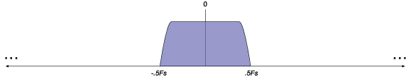
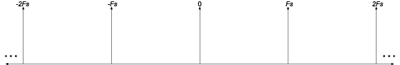
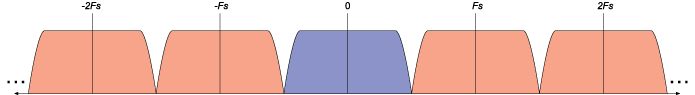
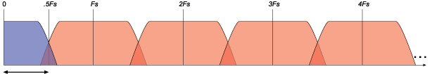
1) Insert a zero between existing samples. (This is the upsampling step, doubling the sample rate and doubling the usable audio bandwidth, but leaving an alias of the original signal in the upper half of the widened audio band.)
2) Remove the aliased image with a lowpass filter. (You can also view this as interpolating between existing samples in the time domain.)
Removing needless calculations
When we implement these two steps, using our FIR filter, we see that every other multiply is by zero, and can be skipped. So, we can omit the zero-insertion step altogether, and just alternate between using the odd and even coefficients on our exiting samples.
You can either index through the coefficients table by steps of two, or split the table into two tables—off and even. This is often called a “polyphase” implementation.
Our 2x oversampling task comes down to this:
1) Buffer enough of the input samples to allow for room to run the FIR filter over the required number of samples.
2) For the current sample, and each new sample that comes in, generate two new samples for the output buffer by applying the odd (ordinal—first, third, fifth…) samples, then the even.
A sketch of the code
In C, we’d do something like this for each new input sample, creating two new output samples:
double coefs[] = { -0.000649, -0.001047, 0.003211, 0.010679,
  0.005956, -0.022766, -0.049404, -0.013106, 0.116023, 0.276227,
  0.349750, 0.276227, 0.116023, -0.013106, -0.049405, -0.022766,
  0.005956, 0.010680, 0.003211, -0.001047, -0.000649 };
long coefsLen = sizeof(coefs) / sizeof(*coefs);   // count 'em

for (n = 0; n <= 1; n++) {      // twice: starting at 1st, then 2nd
  index = indexOfLastSample;    // start at the most recent sample
  double outVal = 0;
  for (m = n; m < coefsLen; m += 2)        // for every other coef
    outVal += inBuf[index--] * coefs[m];   // multiply accumulate

  WriteOutput(outVal);	        // output the new sample
}
Of course, you must ensure that inBuf contains enough samples ((coefLen + 1) / 2). Most likely, you’ll use a circular buffer, so you’ll need to test index for less than zero and wrap around when needed. For instance:
for (m = n; m < coefsLen; m += 2) {    // for every other coef
  outVal += inBuf[index] * coefs[m];   // multiply accumulate
  if (--index < 0)
    index += inBufLength;              // wrap buffer index
}
This example uses a very small filter length (21), and the number of digits in each have been reduced by rounding, in order to allow for a smaller listing, so this is not a high-quality example. But you can substitute a filter of any length for high-quality results.
Additional notes on our filter implementation
When upsampling, signal energy gets distributed over the aliased images, so we must compensate to maintain the signal gain in the region of interest. This means we’ll need a gain of two when doubling the sample rate, and it’s convenient to build it into the coefficients. (Another way of looking at the gain loss is to observe that we compensated for DC gain in the coefficients, but recall that we are only using every other coefficient for each output sample—we need to double it to get back to unity gain.)
Our coefficient calculator always generates an odd number of coefficients. The reason is that we’d like to use an odd-length filter is that the center aligns with a sample exactly, giving us an integer number of samples of delay at the output. We could just as easily generate a windowed sinc that centers between samples for an even number of coefficients, but if we want to align the audio with other samples later, it’s easier to delay in whole numbers of samples than fractions.
The coefficients are always symmetrical, so you don’t need to store the entire table, and you can also take advantage of that symmetry under certain conditions. For instance, in cases where addition is less costly than multiplication, you can add corresponding samples that share the same coefficient value, and save a multiply. This was once a significant optimization, but is usually not an issue with modern processors.
The example shown is written for clarity first, with reasonable performance. You could improve it by using modulo indexing on the input buffer (use a power-of-two sized buffer and AND the index with a mask instead of testing it and wrapping it). You could use a single FOR loop, stepping through the coefficients by one and alternating between output samples. In C++, you could use template meta programming to have the compiler unroll the loops altogether. DSP chips typically combine no-cost modulo indexing with single cycle multiply-accumulate with dual data fetching and zero-cycle looping to result in a cost of one cycle per coefficient.
Depending on quality requirements, we might need a very long list of coefficients. Long convolutions are implemented more efficiently as multiplication in the frequency domain—you could use the FFT to implement the filter.